• Introduction
• what is probabilistic programming
• Why Bayesian
• tutorials
  • simple linear regression
  • multivariate regression (independent predictors)
  • regression with confounds
    • mediator (the pipe)
    • common cause (the fork)
    • the collider
    • multiple confounds all at once
  • categories
  • heterogeneity
  • discrete binary events
• Final thoughts

Introduction

This blog post gives a broad overview of probabilistic programming, and how it is implemented in pymc3, a popular package in Python. As a tutorial, we will go over various basic regression techniques. Meanwhile, we will introduce various concepts in Bayesian probability.

what is probabilistic programming

The goal of probabilistic programming is to implement statistical modeling (mostly Bayesian statistics). My definition for a probabilistic programming is that it is a programming language that deals specifically with random variables. This is in contradistinction to programming language that focus primarily on just variables that are integers or floating numbers.

We can create a random variable object using pure python syntax but it would be quite cumbersome. Here we will use Pymc3 as our probabilistic programming. Pymc3 is a package in Python that combine familiar python code syntax with a random variable objects, and algorithms for Bayesian inference approximation. Beginners might find the syntax a little bit weird. This syntax is actually a feature of Bayesian statistics that outsiders might not be familiar with.

But way of illustration, let us look at a comparison example:

# adding 2 integers in Python
a = 2
b = 3
c = a + b
print(c)

In Pymc3, we can create a random variables that can come from many kinds of probability distribution. In this case, I’ll choose from normal distribution.

# adding 2 random variables in Pymc3
with pm.Model() as example:
	a = pm.Normal('a',2,0.5)
	b = pm.Normal('b',3,0.2)
	c = pm.Deterministic('c',a + b)
	trace_1 = pm.sample()

The last line pm.sample() execute an Markov chain Monte Carlo (MCMC) algorithm to sample values from the distribution. This algorithm numerically approximates values of our variables. MCMC is a workhorse underlying most probabilistic programming languages.

The result that we get is a probability distribution of c.

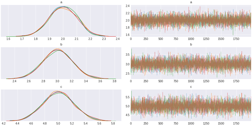
Figure 1.addition of 2 random variables

Another thing you can do with pymc3 is to infer what values of random variables world be, given the data you see. Think about a coin, it looks kinda like a fair coin, but if you see it lands head 8 out of 10, do you still think it fair? So we want to infer the probability of landing head given the observation. You can do that here.

# calculating posterior distribution
with pm.Model() as example2:
	p = pm.Beta('a',1,1)
 	likelihhod = pm.Binomial('likelihood',n = 10,p=p,observed=8)
  	trace_2 = pm.sample(2000,cores=4)

Figure 2. inferring probability of coin toss 8 heads out of 10 trials

So in general, there are two directions you can do with probabilistic programming. You can use it to generate a distribution; or infer a distribution from data. A helpful analogy is a deep learning model, where you have forward and backward propagation. Here you have forward propagation which is generating distribution, and backward propagation being updating the values of your random variables from observation.

One thing to note from the aboved example is that the variablep representing the belief about a coin is a probability distribution called prior distribution. The observed data given the prior is called likelihood (likelihood is itself an unfortunately confusing term that we inherit from frequentist statistics) which is also a probability distribution. The key point here is that they are not different kinds of objects. They are both probability distribution.

This part of Bayesian statistics is what make the pymc3 syntax quite puzzling to beginners. How could our our prior (which is akin to a parameter in the model) and our observed data be represented by the same kind of thing?

One answer is to think that the observed outcome is generated from a random process, and itself can generate random effect (we will later represent this process as a graph). In the grand scheme, we have a chain of random processes. Some of these links in the chain, we can observe, and some we cannot. In the steps we can observe, we can incorporate the observation to the parameters. If not, then the parameter is just a placeholder for our belief of what the process might be like.

What’s more, we can use the observed data as a prior for some unobserved parameter, which in turn is a prior for some observed data. In the unfortunate terminology we inherit, we would say “the likelihood becomes a prior of another prior”. The point is the interchangeability between the observed data and the parameter. This is the basis of hierarchical modeling.

With these in minds, now we can deep dive into the statistics part.

Why Bayesian

tutorials

You might ask “what can you really do in Pymc3?” So this section is about some simple things you can do. The keypoint is using a random variables in the model is a way of putting your uncertainty in the model. You can use random variables in mechanistic models or regression models. You can add random variables in a chain of regression equations. You can even use random variables in a neural network model. But in this blog, we’ll stick to just regressions for now.

This tutorial will start off with a data generation from probability distributions. The output of the data generation is an observed data. Then we will write pymc3 codes to do inference and recover the data generating process. During this, we will reason our ways through what models to use, how to capture the data generating process.

import numpy as np
import pandas as pd
import matplotlib.pyplot as plt

!pip install arviz==0.6.1
!pip install pymc3==3.8
!pip install Theano==1.0.4
import arviz
import theano
import pymc3 as pm

simple linear regression

The key here is that effect (dependent variable) is linearly dependent on independent variables.

np.random.seed(2019)
x1 = np.random.normal(loc=10, scale=3, size=100)
noise = np.random.normal(loc=0, scale=0.1, size=100)
beta1 =  5
y1 = beta1*x1 + noise
data = pd.DataFrame({'x1': x1,'y1': y1})

our code for Pymc3 is very simple. We add together the random variables for the baseline (intercept) and the true effect of x. This is just a linear equation. Then we send this as a variable for a normal distribution that has error term as a standard deviation. To get an inference, we add observed data into the model. Then we sample the distribution to see which distribution will fit the observed data.

with pm.Model() as simple_regression_model:
	# data
	x1 = pm.Data('x1',data['x1'].values)
	y1 = pm.Data('y1',data['y1'].values)

	# prior
	alpha = pm.Normal('intercept',0,10)
	beta = pm.Normal('coeff',0,10)
	sigma = pm.Exponential('error',lam=1)

	mu = alpha + beta*x1

	y_hat = pm.Normal('y_hat',mu,sigma,observed=y1)

	trace_simple_regression = pm.sample(draws=1000,tune=1000)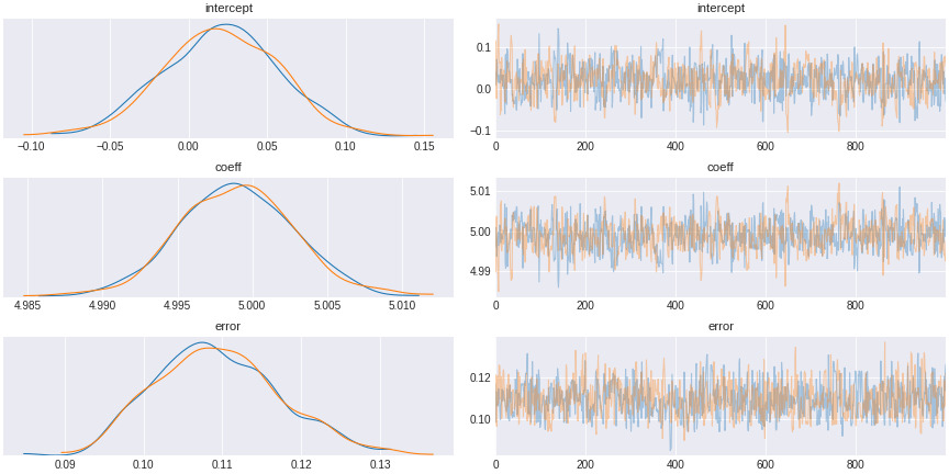

Figure 3. simple Bayesian regression result

The result of this sampling by MCMC is a trace (shown in the right). The trace is a chain of succesive sampling of distribution. On the left we plot the values in the trace as a distribution. We see here that the distribution averaged around 5, the value of the regression coefficient.

multivariate regression (independent predictors)

The multivariate example is just as easy.

np.random.seed(2019)
beta1 = 2
beta2 = 5
x1 = np.random.normal(loc=10, scale=3, size=100)
x2 = np.random.normal(loc=10, scale=3, size=100)
y1 = beta1*x1 + beta2*x2 + np.random.normal(loc=0, scale=0.1, size=100)
data = pd.DataFrame({'x1': x1,'x2': x2,'y1': y1})

To do this in Pymc3, we will write down the equation that generate the outcome and use the same trick.

with pm.Model() as independent_regression_model:
	# data
	x1 = pm.Data('x1',data['x1'].values)
	x2 = pm.Data('x2',data['x2'].values)
	y1 = pm.Data('y1',data['y1'].values)

	# prior
	alpha = pm.Normal('intercept_1',0,10)
	beta_1 = pm.Normal('coeff_1',0,10)
	beta_2 = pm.Normal('coeff_2',0,10)
	sigma = pm.Exponential('error',lam=1)

	mu = alpha + beta_1*x1 + beta_2*x2
	y_hat = pm.Normal('y_hat',mu,sigma,observed=y1)

	trace_independent_regression = pm.sample(draws=2000,tune=1000)

Again the plot shows we can infer back the coefficient values of the regression.

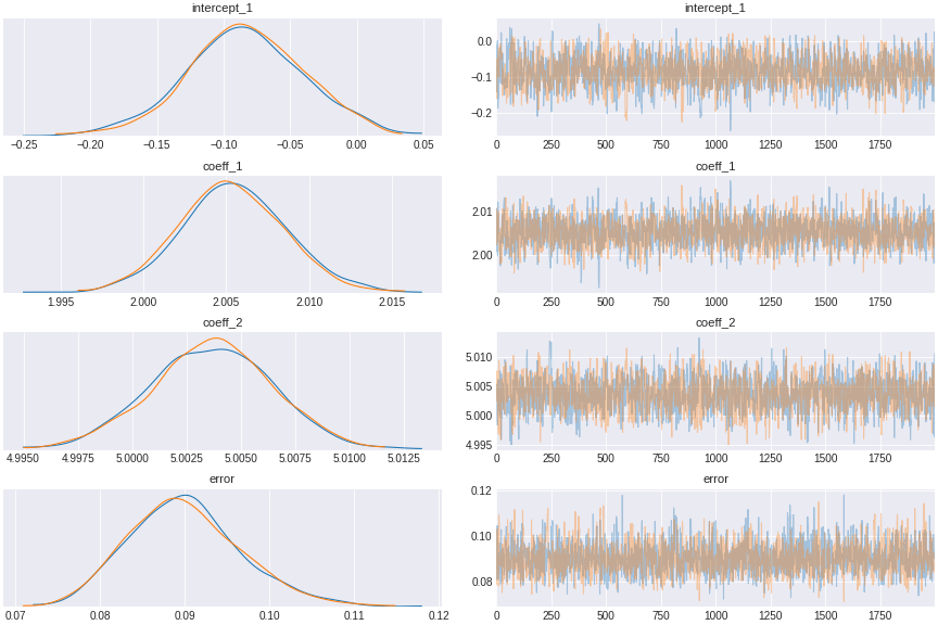
Figure 4. multivariate Bayesian regression result

regression with confounds

The DAGs (directed acyclic graphs) help us visualize the data generating processes. The forward arrow represents how the indepdendent variables (predictors) affect the dependent variables, i.e. the arrow represents the causality. In reality there are many other variables (confounds) that influence dependent variables; and choosing which one to include in the inference can make a difference.

Experiments such as randomized controlled trial is a way of eliminating confounds. But in many cases, one cannot do controlled experiments and has to rely on given data. This is where we can use regression analysis to control for confounds.

There are 4 main types of confounders. Here we’re going to talk about 3 of them.

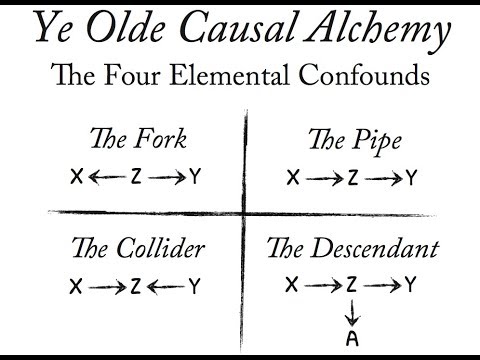
Figure 5. 4 olde causal confounds: the fork, the pipe, the collider, and the descendant. credit: statistical rethinking course by Richard McElreath

mediator (the pipe)

This is a causal process where our independent variable x1 causes some confound x2 that in turn causes y (x1 itself doesn’t cause y). You have to include this type of confound in the model (this technique is known as controlling for a variable).

here is the sample data.

np.random.seed(2019)
beta1 = 2
beta2 = 5
x1 = np.random.normal(loc=10, scale=3, size=100)
x2 = x1 * beta1  + np.random.normal(loc=0, scale=0.1, size=100)
y1 = beta2*x2 + np.random.normal(loc=0, scale=0.1, size=100)
data = pd.DataFrame({'x1': x1,'x2': x2,'y1': y1})

And here is one way to deal with it. You control for a confounding variable.

with pm.Model() as pipe_confound:
	# data
	x1 = pm.Data('x1',data['x1'].values)
	x2 = pm.Data('x2',data['x2'].values)
	y1 = pm.Data('y1',data['y1'].values)

	# prior
	alpha_1 = pm.Normal('intercept_1',0,10)
	beta_1 = pm.Normal('coeff_1',0,2)

	beta_2 = pm.Normal('coeff_2',0,2)
	sigma = pm.Exponential('error_2',lam=1)


	mu = alpha_1 + beta_1*x1 + beta_2*x2
	y_hat = pm.Normal('y_hat',mu,sigma,observed=y1)

	trace_pipe_confound = pm.sample(draws=1000,tune=1000)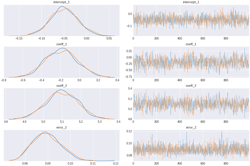

Figure 6. regression control for pipe confound

Another way to do it is to think about generating process. You want to model the causal process how x1 generate x2 and x2 generate y. What you’d want is to do a chain of bayesian regressions. like this.

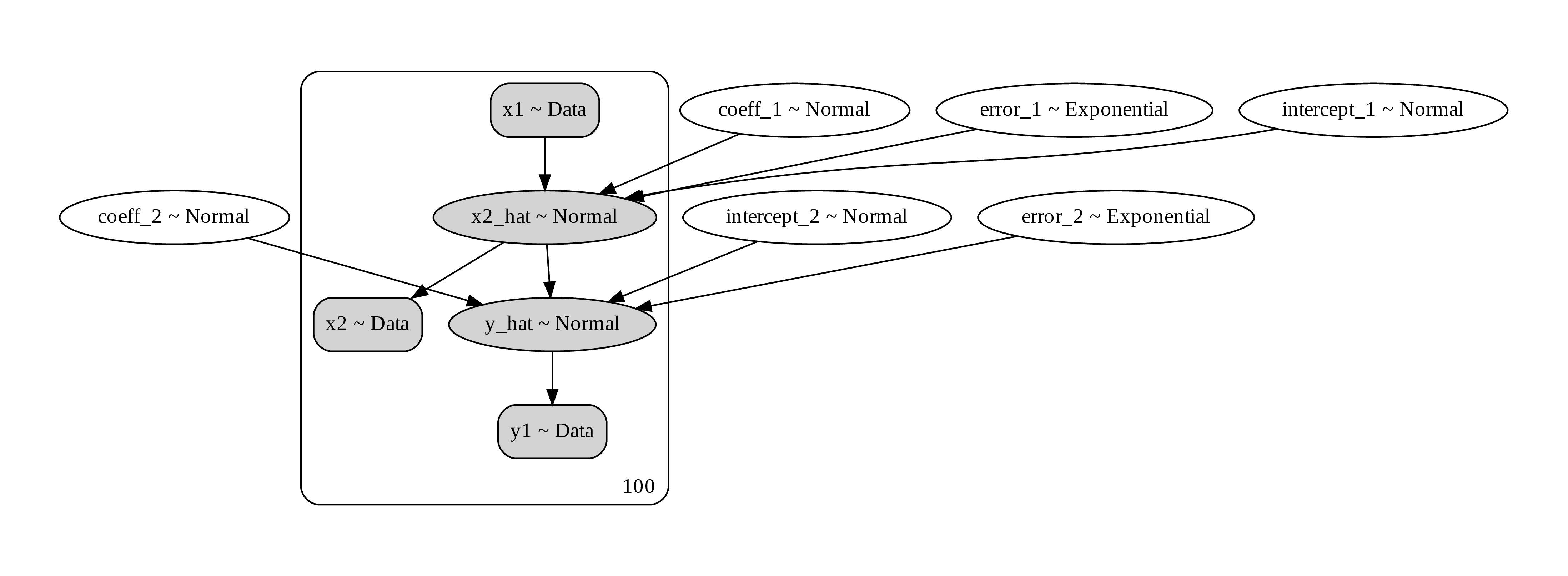
Figure 7. a computational graph of the path analysis showing the prior, the data, and the random distribution that generate them

with pm.Model() as path_analysis_model:
	# data
	x1 = pm.Data('x1',data['x1'].values)
	x2 = pm.Data('x2',data['x2'].values)
	y1 = pm.Data('y1',data['y1'].values)

	# prior
	alpha_1 = pm.Normal('intercept_1',0,10)
	beta_1 = pm.Normal('coeff_1',0,2)
	sigma_1 = pm.Exponential('error_1',lam=1)

	alpha_2 = pm.Normal('intercept_2',0,10)
	beta_2 = pm.Normal('coeff_2',0,2)
	sigma_2 = pm.Exponential('error_2',lam=1)

	mu_1 = alpha_1 + beta_1*x1
	x2_hat = pm.Normal('x2_hat',mu_1,sigma_1,observed=x2)

	mu_2 = alpha_2 + beta_2*x2_hat
	y_hat = pm.Normal('y_hat',mu_2,sigma_2,observed=y1)

	trace_path_analysis = pm.sample(draws=1000,tune=1000)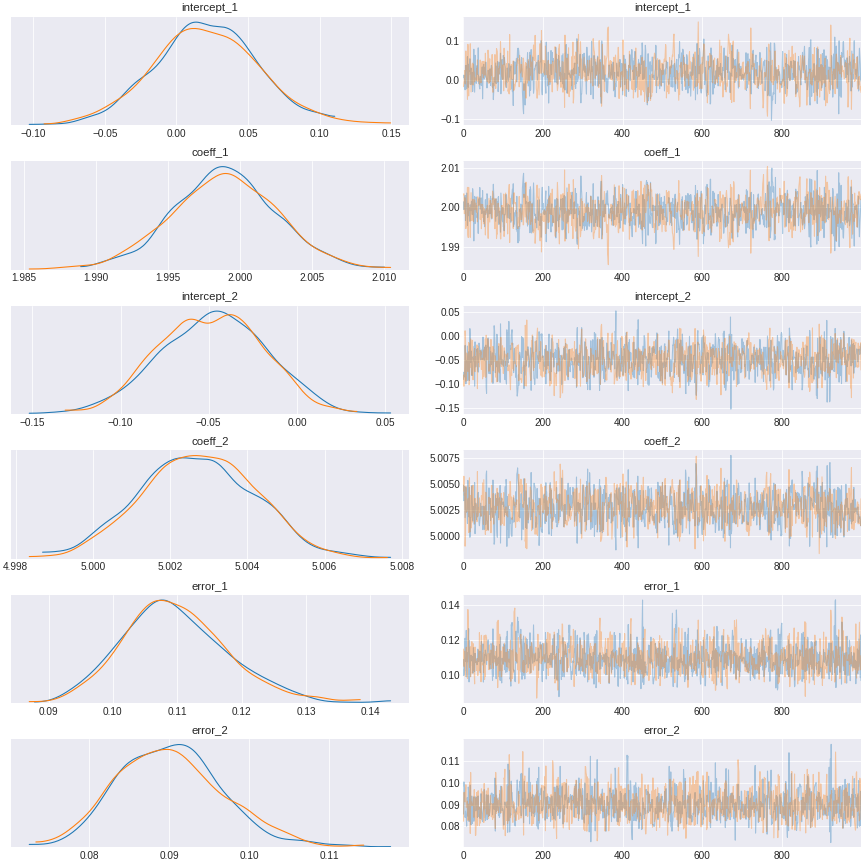

Figure 8. path analysis regression result

In reality, to know which variable is a confound requires understanding of the subject matters, i.e. scientific knowledge. What I show here is how to do the calculation once you identify the confound.

common cause (the fork)

This happens when a confound z causes x1 and y. x1, however, has no causal influence on y.

np.random.seed(2025)
beta1 = 3
beta2 = 2
z = np.random.normal(loc=10, scale=3, size=1000)
x = z*beta1 + np.random.normal(loc=0, scale=0.1, size=1000)
y = beta2*z + np.random.normal(loc=0, scale=0.1, size=1000)
data = pd.DataFrame({'x':x,'z': z,'y': y})

First let’s try fitting a model that doesn’t include confound.

with pm.Model() as no_fork_model:
	x = pm.Data('x',data['x'].values)
	y = pm.Data('y',data['y'].values)

	#alpha = pm.Normal('intercept',0,2)
	alpha = pm.Normal('intercept',0,1)
	beta = pm.Normal('slope',0,1)
	sigma = pm.Exponential('error',lam=1)

	mu = alpha + beta*x
	y_hat = pm.Normal('y_hat',mu,sigma,observed=y)
	trace_no_fork = pm.sample(500,tune=1500,chains=2, cores=2, target_accept=0.95)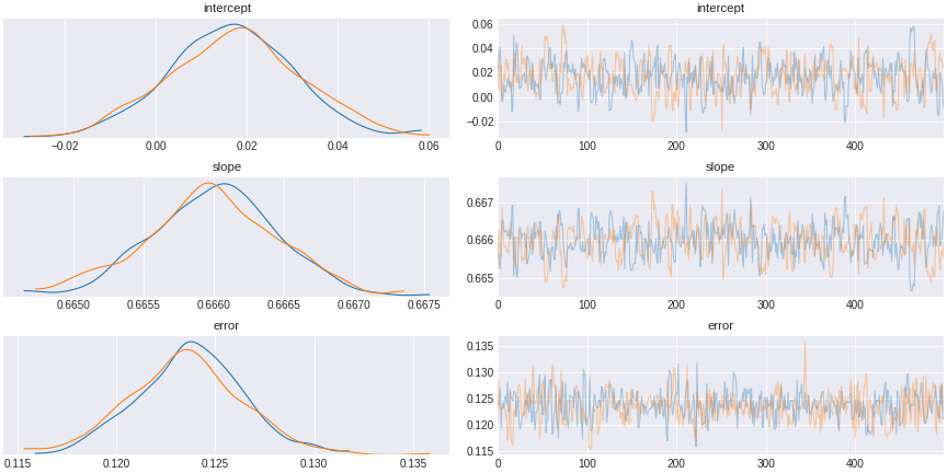

Figure 9. a model that does not control for a confound

What we see is that if we do not include the common cause, we observe spurious correlation that might have led us to think the correlation implies causation.

Now we can try again with model that correctly specify the confound in the regression.

with pm.Model() as fork_model:
  x = pm.Data('x',data['x'].values)
  z = pm.Data('z',data['z'].values)
  y = pm.Data('y',data['y'].values)

  #alpha = pm.Normal('intercept',0,2)
  alpha = pm.Normal('intercept',0,1)
  beta_x = pm.Normal('slope_x',0,1)
  beta_z = pm.Normal('slope_z',0,1)
  sigma = pm.Exponential('error',lam=1)

  mu = alpha + beta_x*x + beta_z*z
  #mu = pm.Deterministic('mu',alpha + beta_x*z + beta_z*z)
  y_hat = pm.Normal('y_hat',mu,sigma,observed=y)#-mu + sigma)
  trace_fork = pm.sample(500,tune=1500,chains=2, cores=2, target_accept=0.95)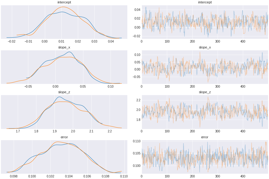

Figure 10. a model controlled for a fork confound

We see that the coefficient of x (slope_x) encompasses 0, indicating that x has no direct causal effect on y.

the collider

This type of confounding is interesting (note that some people don’t call this a confounder, but just a collider). This is when our independent variable x and our dependent variable y causes some variable z. x and y may not have causal relation, but they are correlated through z. To get a correct estimate of x and y, you have to exclude the collider (that’s why some people separate collider from other types of confounders).

The intuition here is to think about a light switch that control a light bulb. If you see the light on, you know the switch must be on and electricity is running in your house. If you don’t see the light on and you see the switch on, then you know the electricity is down in the house. And if you know electricity is running but the light bulb is off, then you know the swich must be off. So there is a correlation between the switch on or off and the electricity running or not through the light bulb. This correlation however is not a causal relation. You cannot infer the causality between the light switch and the electricity.

np.random.seed(2025)
beta1 = 3
beta2 = 2
x = np.random.normal(loc=10, scale=3, size=100)
y = np.random.normal(loc=2, scale=3, size=100)
z = x*beta1 + y*beta2 + np.random.normal(loc=0, scale=0.1, size=100)
data = pd.DataFrame({'x':x,'z': z,'y': y})

Let’s specify a wrong model that include a collider and see.

with pm.Model() as include_collider_model:
	x = pm.Data('x',data['x'].values)
	z = pm.Data('z',data['z'].values)
	y = pm.Data('y',data['y'].values)

	alpha = pm.Normal('intercept',0,1)
	beta_x = pm.Normal('slope_x',0,1)
	beta_z = pm.Normal('slope_z',0,1)
	sigma = pm.Exponential('error',lam=1)

	mu = alpha + beta_x*x + beta_z*z
	y_hat = pm.Normal('y_hat',0,sigma,observed=y-mu)
	trace_include_collider = pm.sample(500,tune=1500,chains=2, cores=2, target_accept=0.95)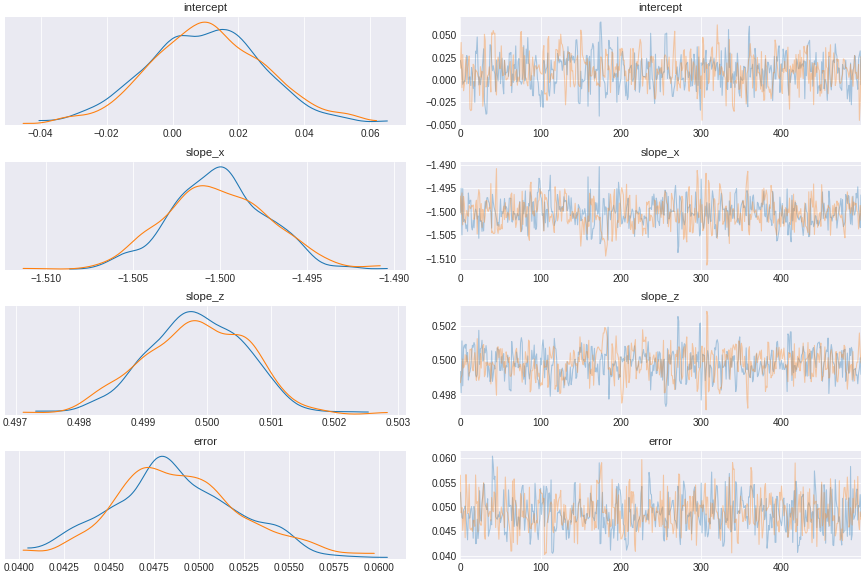

Figure 11. a model incorporating collider

The result shows x and z seemingly excert opposite causal effect on y, when in fact x has no effect on y.

and here is the correct model that exclude collider.

with pm.Model() as exclude_collider_model:
	x = pm.Data('x',data['x'].values)
	y = pm.Data('y',data['y'].values)

	alpha = pm.Normal('intercept',0,1)
	beta_x = pm.Normal('slope_x',0,1)
	sigma = pm.Exponential('error',lam=1)

	mu = alpha + beta_x*x
	y_hat = pm.Normal('y_hat',0,sigma,observed=y-mu)
	trace_exclude_collider = pm.sample(500,tune=1500,chains=2, cores=2, target_accept=0.95)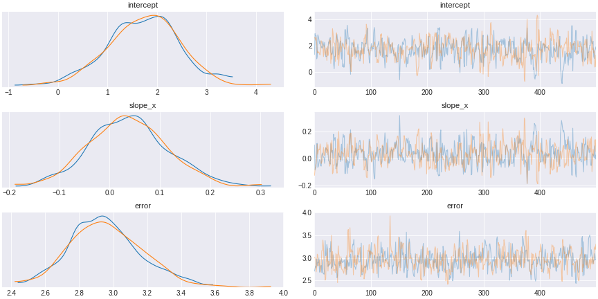

Figure 12. a model excluding collider

multiple confounds all at once

In reality, we work with multiple sources of confounds. Here I simulate a case where we have both a pipe and a collider.

np.random.seed(2025)
beta1 = 3
beta2 = 2
beta3 = -2
beta4 = -1
beta5 = 5
x1 = np.random.normal(loc=10, scale=3, size=1000)
x2 = x1*beta1 + np.random.normal(loc=0, scale=0.1, size=1000)
y = x1*beta3 + x2*beta2+ np.random.normal(loc=0, scale=0.5, size=1000)
z = x1*beta4 + y*beta5 + np.random.normal(loc=0, scale=0.1, size=1000)
data = pd.DataFrame({'x1':x1,'x2':x2,'z': z,'y': y})

Here is how we can write down the graph. Notice that x2 is a pipe of x1 to y, but x1 also has a direct path to y as well. Moreover, both x1 and y affects z. In this way, z is a collider of x1 and y.

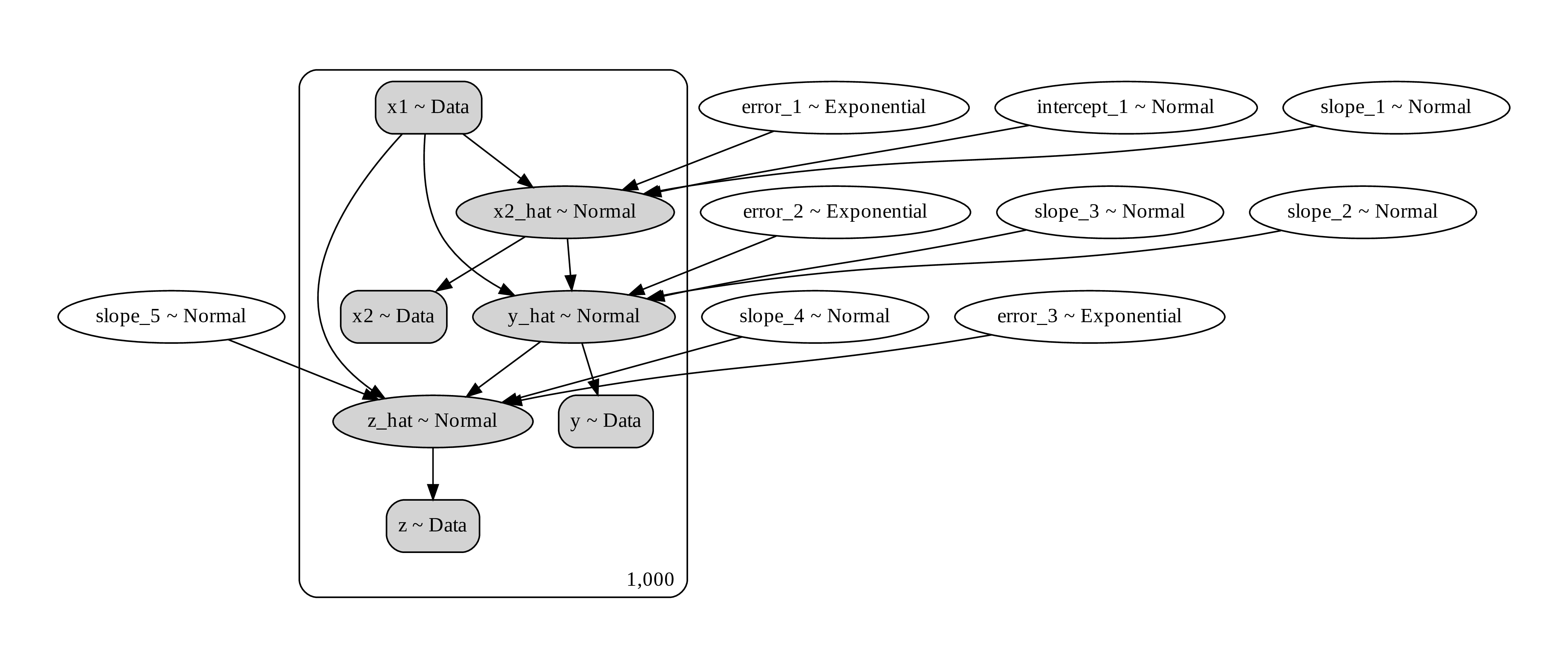
Figure 13. a computational graph representing the causal process

The correct way to do the regression is to exclude z but include x2.

with pm.Model() as combined_model_exclude_collider:
	x1 = pm.Data('x1',data['x1'].values)
	x2 = pm.Data('x2',data['x2'].values)
	y = pm.Data('y',data['y'].values)

	#alpha = pm.Normal('intercept',0,2)
	alpha_1 = pm.Normal('intercept_1',0,1)
	beta_1 = pm.Normal('slope_1',0,1)
	beta_2 = pm.Normal('slope_2',0,1)
	beta_3 = pm.Normal('slope_3',0,1)

	sigma_1 = pm.Exponential('error_1',lam=1)
	sigma_2 = pm.Exponential('error_2',lam=1)

	x2_hat = pm.Normal('x2_hat',beta_1*x1 + alpha_1,sigma_1,observed=x2)
	y_hat = pm.Normal('y_hat',beta_2*x2_hat + beta_3*x1,sigma_2,observed=y)
	trace_exclude_collider = pm.sample(500,tune=1500,chains=2, cores=2, target_accept=0.95)

Here is the result after you control for the pipe but exclude the collider

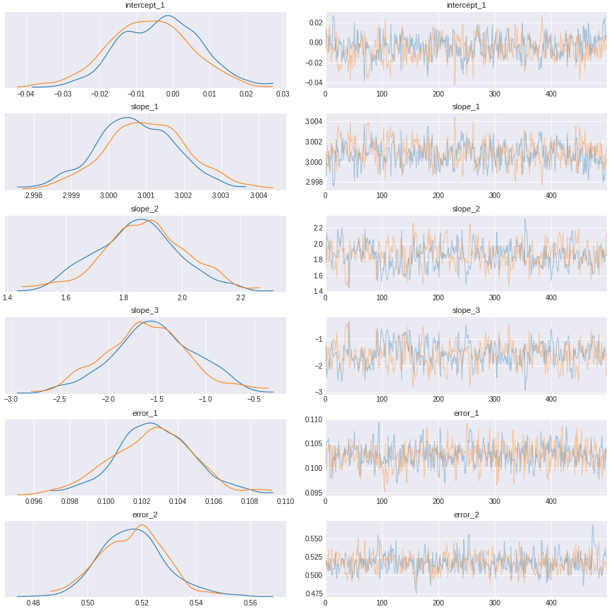
Figure 14. a result of model control for the pipe confound, and exclude the collider

This should give us a flavor of how to use Bayesian regression to investigate causality in the data.

The next part will deal with different types of data, such as count data, and categorical data.

categories

This is a case when we deal with a categorical variables (i.e. unordered class).

np.random.seed(2025)
beta1 = np.random.normal(loc=0, scale=2, size=5)
beta2 = np.random.normal(loc=1, scale=1, size=4)

x1 = np.random.choice(5,size=100)
x2 = np.random.choice(4,p=[0.1,0.2,0.3,0.4],size=100)
y1 = beta1[x1] + beta2[x2] + np.random.normal(loc=0, scale=0.1, size=100)
data = pd.DataFrame({'x1': x1,'x2': x2,'y1': y1})

We have 2 groups of categories: x1 and x2. x1 has 5 classes; and x2 has 4 classes. Instead of specifying 9 random variables, we’ll create 2 tensor objects of random variables with length 5 and length 4. Then use the categorical variables as index to the tensor. The rest is just a regression.

with pm.Model() as categorical_model:
	x1 = theano.shared(data['x1'].values)
	x2 = theano.shared(data['x2'].values)
	y1 = pm.Data('y1',data['y1'].values)

	cat_x1 = pm.Normal('cat_x1',0,1,shape=len(data['x1'].unique()))
	cat_x2 = pm.Normal('cat_x2',0,1,shape=len(data['x2'].unique()))
	sigma = pm.Exponential('error',lam=1)

	mu = cat_x1[x1] + cat_x2[x2] #+ alpha
	y_hat = pm.Normal('y_hat',mu,sigma,observed=y1)
	trace_categorical = pm.sample(500,tune=1500,chains=2, cores=2, target_accept=0.95)

Now one awesome thing that Bayesian analysis can do is to do hierarchical modeling. If you look at the data generation code, you’ll see that effect of category x2 on y are generated from a common distribution. This sometimes is not surprising because different classes in a bigger category probably share some property in common.

with pm.Model() as pooled_categorical_model:
  x1 = theano.shared(data['x1'].values)
  x2 = theano.shared(data['x2'].values)
  y1 = pm.Data('y1',data['y1'].values)

  pooled_x2_mu = pm.Normal('pooled_x2_mu',0,1)
  pooled_x2_sigma = pm.Exponential('pooled_x2_sigma',lam=1)

  cat_x1 = pm.Normal('cat_x1',0,1,shape=len(data['x1'].unique()))
  cat_x2 = pm.Normal('cat_x2',pooled_x2_mu,pooled_x2_sigma,shape=len(data['x2'].unique()))
  sigma = pm.Exponential('error',lam=1)

  mu = cat_x1[x1] + cat_x2[x2]
  y_hat = pm.Normal('y_hat',mu,sigma,observed=y1)
  trace_pooled_categorical = pm.sample(500,tune=1500,chains=2, cores=2, target_accept=0.95)

Here is what the computational graph looks like.

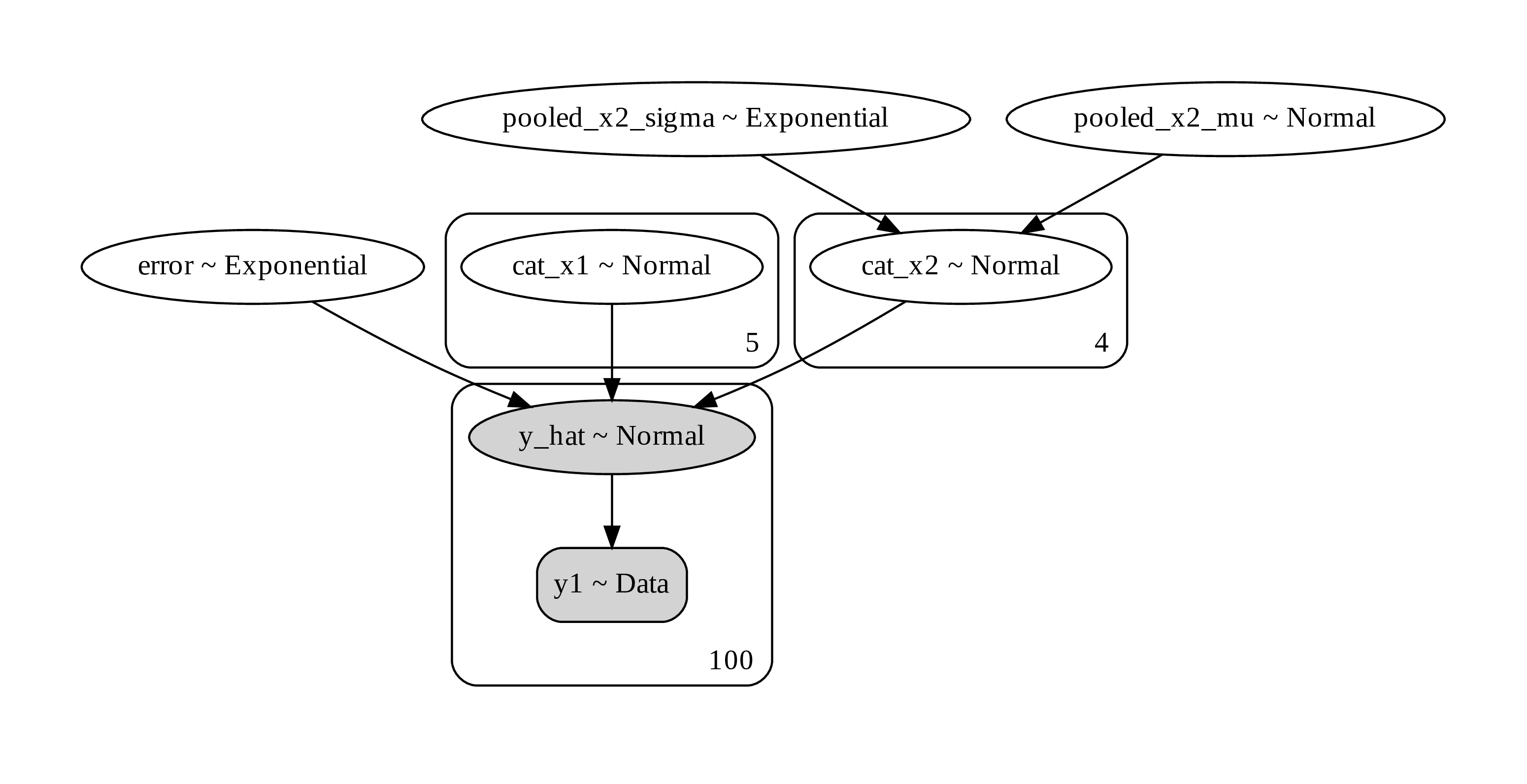
Figure 15. a computational graph of a hierarchical Bayesian modeling

Unlike non-hierarchical modeling where we estimate class parameter separately the hierarchical modeling allows us to pool the effect across class into a higher hierarchical variable. Then each class variable is a variation on the higher variable. This is useful when the the class doesn’t have a lot of samples. Estimating the mean from low samples results in inaccurate estimates. So it may be better to base the low-sample estimate close to the category mean. This is a phenomenon known as shrinkage, also related to “regression to the mean”. what it means is that the estimate of low samples tend to string to towards the category mean.

But why is this useful when we have big data? Because with big data, you can segment the classes further and get a more fine-grain model.

heterogeneity

This is when the effect of one treatment vary in population, i.e. population in different class are affected differently. I wrote a blog post a while ago about how to do this using random forest regression. Now we’re going to try this using Bayesian regression. The key is that we’re going to have a categorical variable for each segment of population.

np.random.seed(2025)
beta3 = np.array([[2,1],[-2.5,2],[-3,3]]) # x1->x2

x1 = np.random.choice(3,size=100)
x2 = np.random.choice(2,size=100)
y1 = beta3[x1,x2] + np.random.normal(loc=0, scale=0.1, size=100)# + beta1[x1] + beta2[x2]
data = pd.DataFrame({'x1': x1,'x2': x2,'y1': y1})

First let’s try it without heterogeneity. We’re estimating the effect of x2 (this could be the treatment) in the population.

with pm.Model() as no_heterogenous_model:
  x1 = theano.shared(data['x1'].values)
  x2 = theano.shared(data['x2'].values)
  y1 = pm.Data('y1',data['y1'].values)

  #alpha = pm.Normal('intercept',0,2)
  cat_x1 = pm.Normal('cat_x1',0,1,shape=len(data['x1'].unique()))
  cat_x2 = pm.Normal('cat_x2',0,1,shape=len(data['x2'].unique()))
  sigma = pm.Exponential('error',lam=1)

  mu = cat_x1[x1] + cat_x2[x2] #+ alpha
  y_hat = pm.Normal('y_hat',mu,sigma,observed=y1)
  trace_no_heterogenous = pm.sample(500,tune=1500,chains=2, cores=2, target_accept=0.95)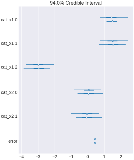

Figure 16. a Bayesian regression model that does not include interaction terms

The interval includes zero, indicating x2 has no effect in the population.

But let’s do it again with heterogeneity included in the model.

with pm.Model() as heterogenous_model:
  x1 = theano.shared(data['x1'].values)
  x2 = theano.shared(data['x2'].values)
  y1 = pm.Data('y1',data['y1'].values) 


  error = pm.Exponential('error',lam=1)

  #these blocks of codes create covariance matrix for every x1,x2 pairs
  # Compute the covariance matrix
  a_bar = pm.Normal('a_bar', mu=0, sd=2)
  b_bar = pm.Normal('b_bar', mu=0, sd=2)
  sigma = pm.Exponential.dist(lam=1)
  packed_chol = pm.LKJCholeskyCov('chol_cov', eta=2, n=2, sd_dist=sigma)
  chol = pm.expand_packed_triangular(2, packed_chol, lower=True)
  cov = theano.tensor.dot(chol, chol.T)
  # Extract the standard deviations and rho
  sigma_ab = pm.Deterministic('sigma_ab', tt.sqrt(tt.diag(cov)))
  corr = theano.tensor.diag(sigma_ab**-1).dot(cov.dot(theano.tensor.diag(sigma_ab**-1)))
  r = pm.Deterministic('Rho', corr[np.triu_indices(2, k=1)])


  ab_cat = pm.MvNormal('ab_did', mu=[a_bar,b_bar], chol=chol, shape=(len(data['x1'].unique()), 
  len(data['x2'].unique())))

  # calculate mean of y_hat from the multivariate Normal distribution
  mu = ab_cat[x1,x2]
  y_hat = pm.Normal('y_hat',mu,error,observed=y1)
  trace_heterogenous = pm.sample(500,tune=1500,chains=2, cores=2, target_accept=0.95)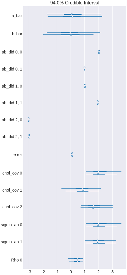

Figure 17. a Bayesian regression model including interaction terms for heterogeneity

Now you see that the effect of x2 vary among x1 classes. The overall effect is zero because the overall effect among classes cancels out.

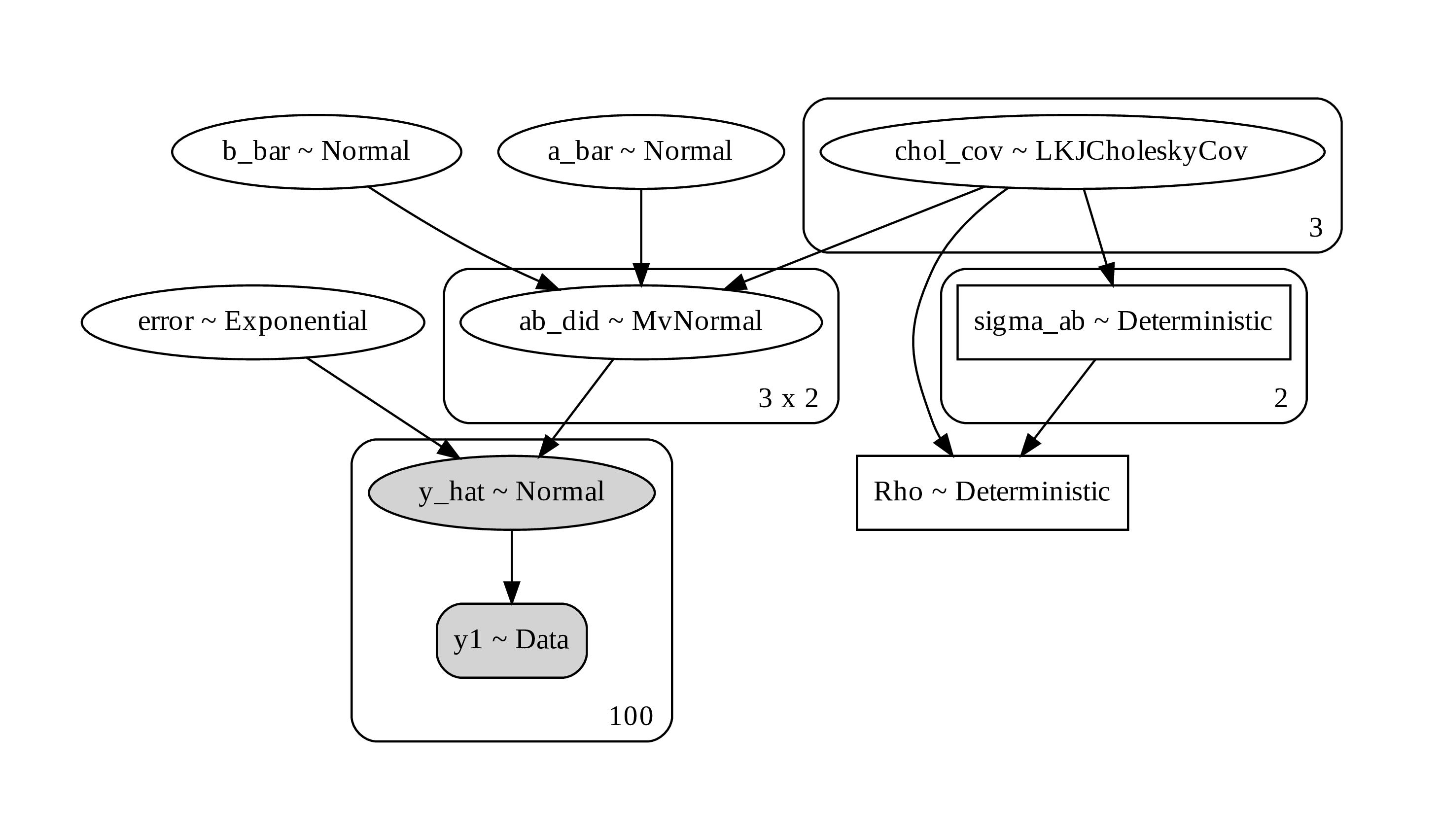
Figure 18. a computational graph for Bayesian regression with heterogenous effect

In the code, I include the use of LKJCholesky matrix. This matrix is used as a prior for multivariated normal distribution. You may not need to use it. Using a saparated value for each prior in univariate Gaussian can give you a result as well.

discrete binary events

This is when the outcome is a binary result of a probability trial, and we want to know the probability of getting the outcome. A helpful analogy is a coin toss with fix unknown probability of landing head. Then we can model how different variables affect the probability. A typical problem is how a treatment affects the underlying probability that lead to the observed events.

np.random.seed(2020)
beta3 =  np.array([[0.1,0.2],
                  [0.2,0.1],
                  [0.3,0.3]])

x1 = np.random.choice(3,size=10000)
x2 = np.random.choice(2,size=10000)
p1 = beta3[x1,x2]
y1 = np.random.binomial(1,p1,size=10000)
data = pd.DataFrame({'x1': x1,'x2': x2,'y1': y1})
data.tail()

To model this, we simulate drawing an event from Bernoulli distribution, where the probability is a random variable we’re interested in. This could be an effect of new treatment (x2) given to a heterogenous (x1) population. The outcome is binary (such as purchased or not purchased, or death or not alive)

Let’s do it with heterogeneity added as interaction term. There are many ways to do this, one can logistic regression and do inverse logit to get a probability (p), and send the probability p to Bernoulli process. Alternatively, we will use a flat beta distribution as a prior to the Bernoulli process.

with pm.Model() as count_heterogenous_model:
  x1 = theano.shared(data['x1'].values)
  x2 = theano.shared(data['x2'].values)
  y1 = theano.shared(data['y1'].values) 

  # prior
  prob1 = pm.Beta('treatment effect',alpha=1,beta=1,shape=(3,2))
  # likelihood
  y_hat = pm.Bernoulli('y_hat',p = prob1[x1,x2],observed=y1)
  diff = pm.Deterministic('diff', prob1[:,1] - prob1[:,0])
  trace_count_heterogenous = pm.sample()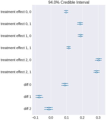

Figure 19. a model for Bernoulli process

Final thoughts

There are still many more tutorial examples that I think would be fun to go over. We still haven’t touched on a lot of interesting topics. So this will be my future work on the probabilistic programming tutorial. I plan to include topics such as missing data, survival analysis, ordered categorical variables, basic time series, combining Bayesian statistics with ordinary differential equations, and finally deep probabilistic learning where we combine probabilistic programming with deep learning.