Heterogenous effects estimation using Causal Tree Analysis
Heterogenous Effect
In my last month blog post I discussed using Bayesian MCMC technique to quantify the effect of an online ad. One important thing that I should point out right away is that the effect is at the population level. It is likely that in reality the respond to a treatment (an ad) is heterogenous; that is to say, some sectors of the population are more responsive than others. Possibly, some might respond negatively.
This might not be such a big problem for certain forms of online ads such as email ad, because the cost of an ad is minute. However, it can post a serious problem for something costly or can have negative effect. Take a drug treatment example. It is possible that a drug can have deleterious effect to certain patients. Therefore it becomes necessary to catch the heterogenous effect in the population.
So in this blogpost, we will explore one simple method called “causal tree” to isolate the sub-population that are more responsive positively or negatively through a simple medical treatment example. But keep in mind that this can be generalize to other domains such as online ads, user interaction with products, etc.
What is Causal Tree?
Causal tree is a non-parametric estimation of heterogenous treatment effects using a decision tree technique (I will probably do a blogpost on this technique later). Causal forest is when many decision trees (random forest) are generated. It should be noted though that Python does not have a good package to do full a causal tree analysis, and I know some people use R to do this type of work. But for the educational purpose here, I will use a very simple example that simple Python code can work with. Now let’s deep dive into it.
Randomized Control Trial
Our example describe a plausible scenario of medical drug randomized control test, where we have 100000 patients, half of which receive a placebo drug, and the other half receive the drug treatment. We also collect attributes of the patients. In our case, the attributes are weight, height, and gender. We then look at the outcome whether the treatment cures the illness or not.
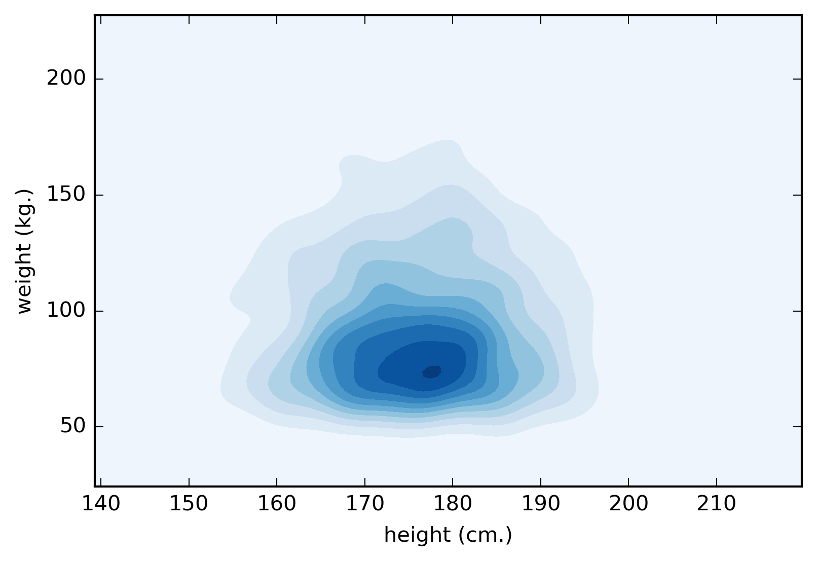
Figure 1. A contour plot representing the distribution of patients height and weight.
Now suppose that each patient has a propensity to overcome the illness. And the environmental effect, including the treatment, either enhance or diminish this propensity. However, this propensity is hidden from us. All we know is whether the patient overcome the illness or not. At the population level, without treatment, we will measure this as the baseline probability of recovery. In my example, I will simulate the data such that the baseline probability of recovery is around 0.4. That is without drug, the baseline recovery is normally distributed around 0.4.
Now, in this example, the drug will increase the probability to 0.7 only among patients with body mass index (BMI) lower than 24 (about healthy mass-height proportionality). But the drug also will harm patients with BMI greater than 24 in that it lowers the probability of recovery from the illness to about 0.2. At the population level though, the measured effect of the drug will be somewhere between 0.7-0.2 depending on the demographic of the patients receiving the treatment. Again the propensity associated with each individual is hidden from us, and all we can observe is at the aggregate level how many patients are cured, and what attributes indicate good prognosis, and what attributes are contraindications (i.e. indicates bad prognosis). And it is the task to isolate the attributes of the sub-population associated with good prognosis and bad prognosis.
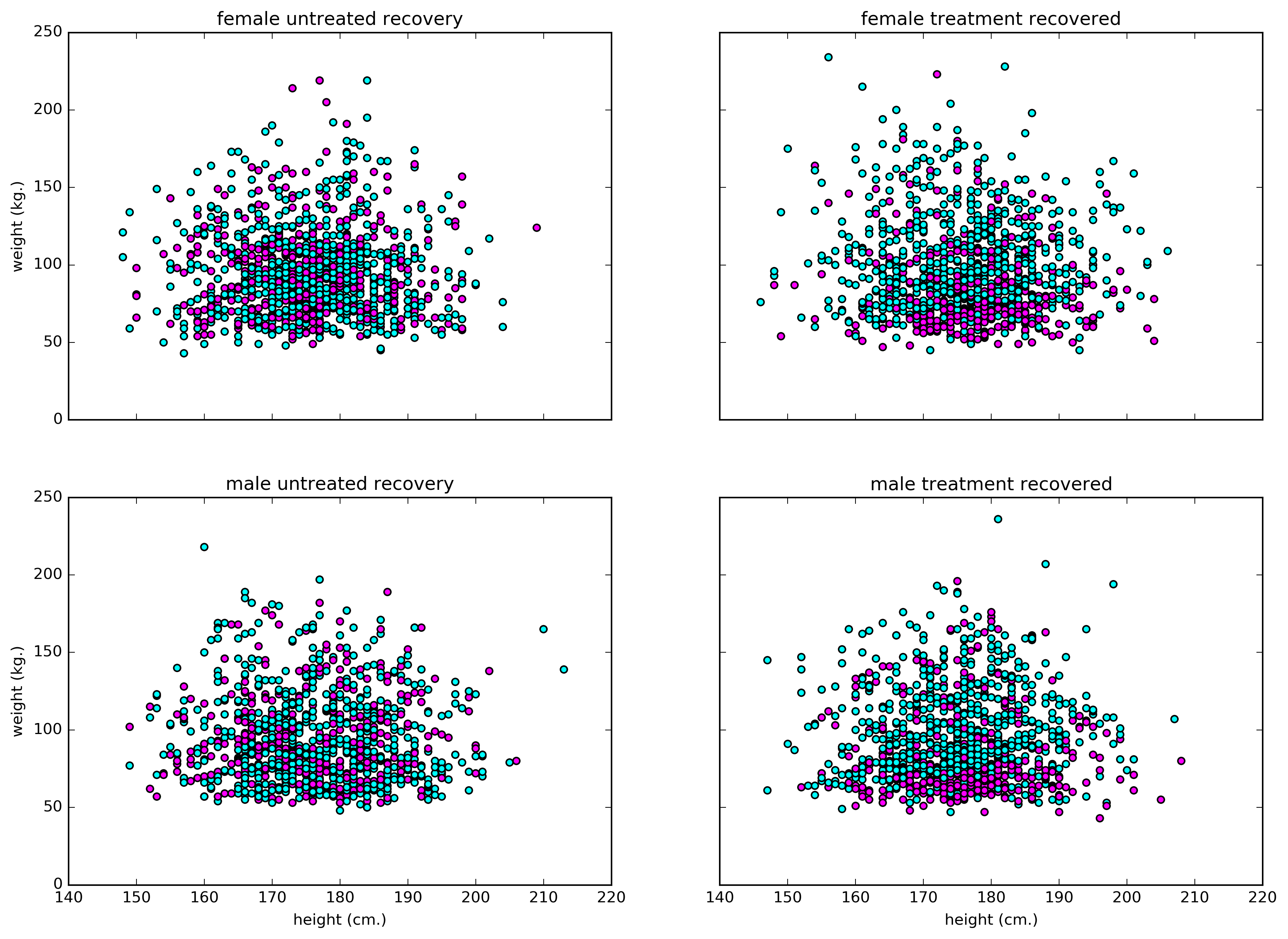
Figure 2. A scatter plot showing recovery of patients categorized by height, weight, and gender. Blue represents not-recovered, and margenta for recovered.
From this dataset, we can calculate following
overall recovery rate = 0.37 baseline recovery probability = 0.40 treatment recovery probability = 0.34 percent efficacy of the drug = -15.68
So, percent efficacy is negative. Does it mean the drug doesn’t help anyone? Not necessarily, it could be that drugs are harmful to most people, but could still be beneficial to some sub-populations. So we will go ahead and implement causal tree to find that sub-population.
How to implement causal tree algorithm
Describe the algorithm
- make a random subsample to divide the dataset into the the training set and the test set.
- Use the attributes in the dataset to train a decision tree regression. the dependent variable is whether the person recover or not, and the regressors are the attributes. The splitting criteria is the squared-error minimization.
- Estimate the leaf-wise response rate from the test set.
- The response rate is determined as the difference between the recovery rate in treatment group and the control group.
Why does it work?
The key assumption is unconfoundedness. This assumption requires the treatment to be random. This essentially means that we can treat nearby points in high dimensional space in the leaf node as a sub-population in a mini randomized experiment. And our leaf-wise estimate will be the efficacy of a randomized control drug trial in that subpopulation sharing particular attributes.
Noted also that this approach requires spliting the dataset into the training set and the estimating set. This is to prevent over-fitting, which will lead to over-estimating or under-estimating the leaf-wise response rate. This might seems like we are throwing away half of the data that could be used for training the tree. But this is just for one decision tree. As dataset gets more complex, we can use random-forest technique, and each time that we sample new training set for a decision tree, we will use all of the data for both splitting and estimation. Just not the same datapoint for the same tree.
What does the tree look like?
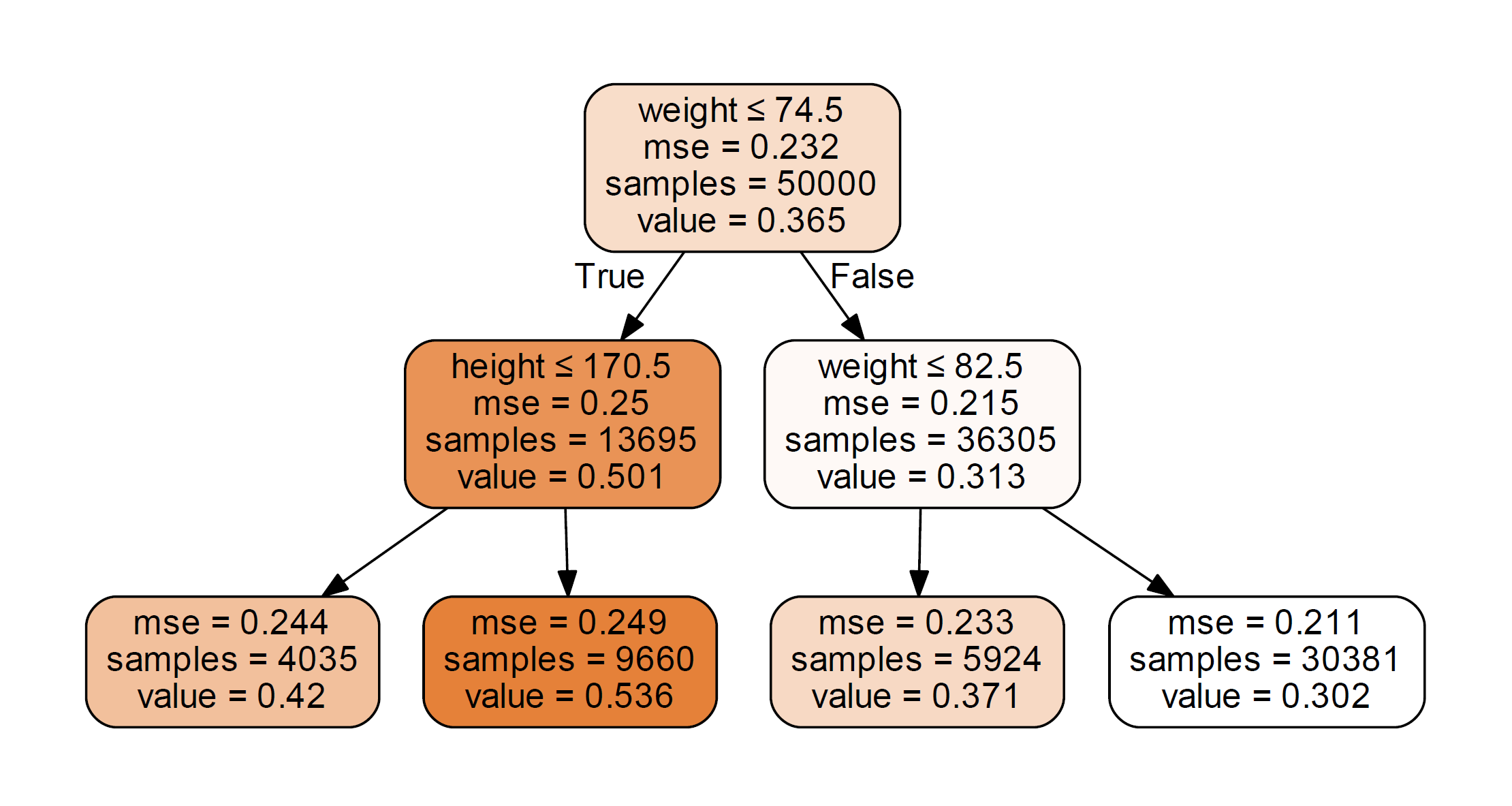
Figure 3. A tree diagram estimating the probability of recovery. The decision rules as well as the mean squared error are shown. The "value" refers to probability of recovery.
Note that in this example, we fit the training set to only one tree with depth = 2. In reality, we would have to try different tree structures. From the figure we can see the decision rules are about weight and height (gender plays no role in it), which is consistent with the way we simulate the data.
Now from this tree structure, we can perform classification on the test set using the tree we just made. The result is shown in the figure below.
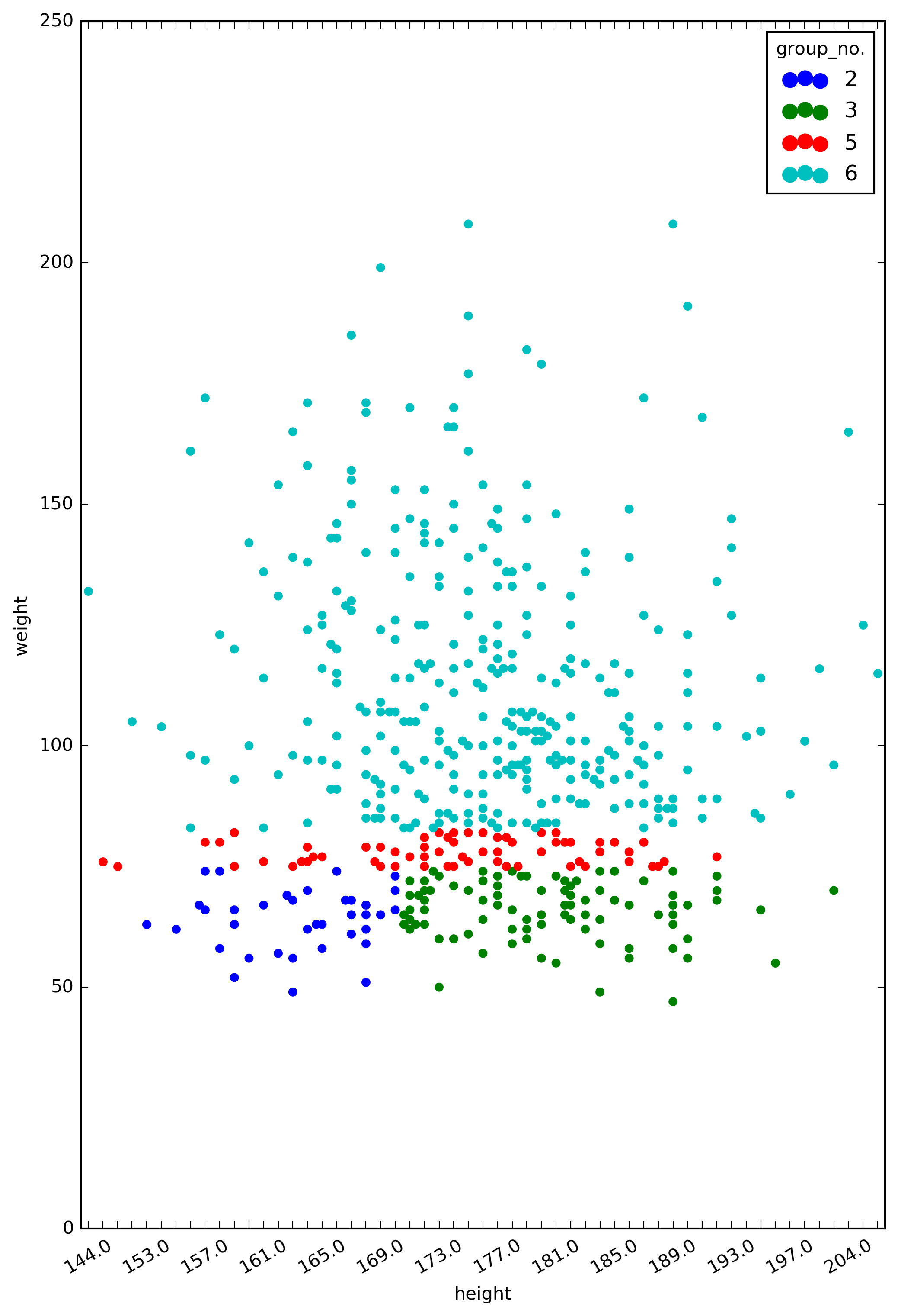
Figure 4. The classes generated from the decision tree.
The groups of colored points represent the subpopulations in our dataset that are classified by the decision tree. Group 3, for example, is a subpopulation of individuals with weight <= 74.5 kg and height > 170.5 cm (which is the bottom right sector of the plot).
Now one last thing we need to do is to simply calculate the responsiveness to treatment for each group. This is just the difference of recovery rate in treatment group and control group.
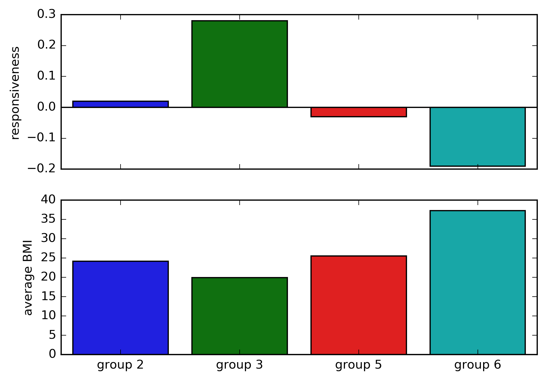
Figure 5. The estimated effect of drugs. The responsiveness is the change in recovery probability in the treatment group compared to the control group. The average body mass index in each group is shown below.
Recall that we created a dataset in which the drug will increase the probability of recovery to 0.7 only among patients with body mass index (BMI) lower than 24. This figure shows that the causal tree analysis seems to be able to capture this effect.
Conclusion
What I see as the advantages is that the causal tree representation is easy implement on expermental data, and results are easy to interpret and explain, especially if the splitting rules have an articulable meaning. The downsides are we often don’t know a priori how many classes we expect, so the depth level of the trees as well as the classes might not have any meaning. This can be dangerous if the trees are over-complex and the results do not generalize well, creating spurious effect wrongly attributed to a small sub-population. In that situation, pruning of trees and using random forests will help with the problem.
