1. background

I took a class in applied machine learning at Cornell Tech last year. One class project that I worked on is to develop an algorithm for image search. In this blog post I will describe how this can be done using simple machine learning tools. First, let’s talk about the task.

The task here is to match images in the database to the search text query. As supervised learning task, we have 10000 images in the training database, and for each image, there are 5 short sentences that describe the image in moderate detail. Furthermore, for each image we have human-labeled tags, that refers to objects/things in the image.

For example,

Figure 1. An example of a training image.

As part of the image, it is tagged with a label:

vehicle:airplane outdoor:bench sports:skateboard person:person vehicle:truck accessory:backpack accessory:handbag furniture:dining table

the image also comes with a 5 short descriptions.

The skateboarder is putting on a show using the picnic table as his stage. A skateboarder pulling tricks on top of a picnic table. A man riding on a skateboard on top of a table. A skate boarder doing a trick on a picnic table. A person is riding a skateboard on a picnic table with a crowd watching.

And our task here is to generate a mapping from a these decriptions to image most associated with the description.

2. ML algorithm

2.1 How to we measure success?

The goal is to retrieve the exact image that matches the description. However, this is unlikely to succeed since the training set is quite small and the images can get complex. More reasonably, we aim to retrieve top 20 relevant images, ranked by the likelihood of matching the descriptions. If score reflects the rank where the retrieved images match the description. The formula is score = 1/(1+n) where n is the rank from 0 to 19. So the highest score for one image is 1 where the first image being retrieved is the correct one.

2.2 the machine learning task

We decided to do supervised learning approach to tackle the problem. we divided the dataset into the holdout validation set, and and the training set. After trying different approaches ranging from nearest neighbors, randomforest, and regularized regression, we dicided to present only the result from the regularized regression. Chosen as a baseline for memory-based lazy learning, Nearest neighbors does not perform as well as other two as it tends to suffer from the curse of dimensionality. While Random Forest may perform well, the fitting takes a really long time. Regularized regression is fastest and yields a reasonably high accuracy score. So in the following paragraphs, we will talk only about the work done by regularized regression. The python codes for this work is hosted on this GitHub.

3. Pre-processing

3.1 ResNet-50

We used a neural network approach called “Residual neural network” or “ResNet” to classify contant appeared in the images. here is the reference. Also see appendix 1 for more explanation.

The pre-trained Resnet model is implemented in Keras package Here (also see the code). We chose Resnet-50 which is pre-trained on a databased “ImageNet”. This ResNet is 50 layers deep and can classify images into 1000 object categories. The output consists objects predicted by the ResNet and the associated probability from the softmax layer. We will need both for the next pre-processing step.

import tensorflow as tf
from keras.applications.resnet50 import ResNet50
from keras.preprocessing import image
from keras.applications.resnet50 import preprocess_input, decode_predictions
resnet_model = ResNet50(weights='imagenet')

img_path = 'data/images_train/1.jpg' # for image 1
img = image.load_img(img_path, target_size=(224, 224))
x = image.img_to_array(img)
x = np.expand_dims(x, axis=0)
x = preprocess_input(x)

preds = resnet_model.predict(x)
print('Predicted:', decode_predictions(preds, top=5)[0]) # get the top 5 objects classified by resnet.
# Predicted: [('n07590611', 'hot_pot', 0.42168963), ('n04263257', 'soup_bowl', 0.28596312), ('n07584110', 'consomme', 0.06565933),  
# ('n07875152', 'potpie', 0.024351457), ('n07579787', 'plate', 0.021794433)]

3.2 fastText

The next step aims at embedding the these object labels to word2vec vectors so that we can use them in our ML models. We decided to use fastText embedding to convert the word strings to vector representation reference. See the appendix 2 for more explanation.

We obtained the pre-trained word2vec model using fastText reference here contains the downloadable pretrained word vectors. we used Gensim package to read and implement the pre-trained English word vectors “cc.en.300.bin”.

To do the embedding, we picked top 5 objects classified by the ResNet-50 ranked by the probability. Then convert each word to 300-dimension vectors and do the weight-sum of these vectors by the probability. The result we have is a 300-dimension vector that represents a weighted average of the objects classified by ResNet.

from gensim.models.wrappers import FastText
fasttextmodel = FastText.load_fasttext_format('cc.en.300.bin')

3.3 TFIDF text embedding

After image embedding, We still have to deal with the sentence descriptions. we decided to use TFIDF embedding to extract the text information. TFIDF is a way of weighing word frequency in documents in the corpus. The formula and rationale behind the formula can be found here. See the appendix 3 for more explanation.

But before we do that , first the text has to be cleaned up a bit. We lowercase all words, remove punctuations, and lemmatize (remove the inflectional suffixes) the words. However, we found that some words still appear in multiple forms. Finally, we use stemming to remove most of the endings from words to get the root form. TFIDF vecterization is performed separately on the description text and the labled tag. This results in a TFIDF document vector of 6837 dimensions for the description corpus, and 101 dimensions for the labeled tag corpus.

4. word2vec from TFIDF

After initial attempt using only TFIDF (see figure 5), we found that many words in the description or the tags appear as synonyms or words with similar meanings, such as a sentence “a man walks behind an ice cream truck” is associated with an image

Figure 2. image of "a man walks behind an ice cream truck".

and is tagged as {vehicle:car, vehicle:truck, outdoor:traffic light, person:person}. Note that the tag does not contain the word “man” but instead use the word “person”. If we have ample amount of data, the regression should be able to detect correlation between the word “man” and the word “person”, however, we decided that to push this task a little further, we perform word embedding using fastText the top words from TFIDF to vector representations. This should allow the synonym words to be embedded as close points in high dimensional vector space. For example, we measure the distance using cosine-similarity. The cosine similarity between “man” and “woman” is 0.77;”man” and “person” is 0.56;”woman” and “person” is 0.56; “man” and “truck” is 0.29; and “truck” and “person” is 0.14.

To obtain the word2vec of the description documents, we perform weighted average of top 15 words in the documents, ranked by their TFIDF scores. The weights for the weighted averaging are the TFIDF scores. Similarly, We did the same with the tags, taking top 5 words for the weighted averaging.

As sanity check, we check the cosine similarity between this description TFIDF-weighted word2vec and the embedding strategy of the image information in 3.2. The median cosine similarity is about 0.47 (figure 2). The median cosine similarity between the description TFIDF-weighted word2vec and the tag TFIDF-weighted word2vec is 0.71 (figure 3).

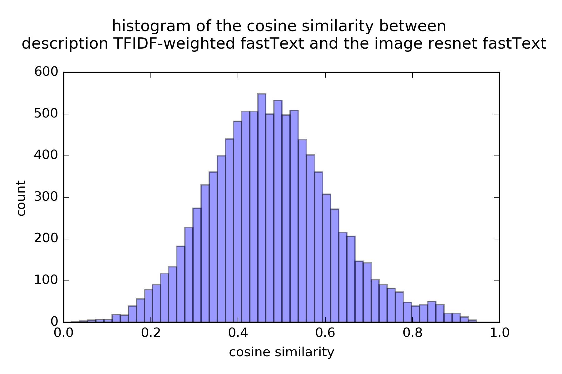
Figure 3.1. similarity between the resnet and TFIDF-weighted fastText.

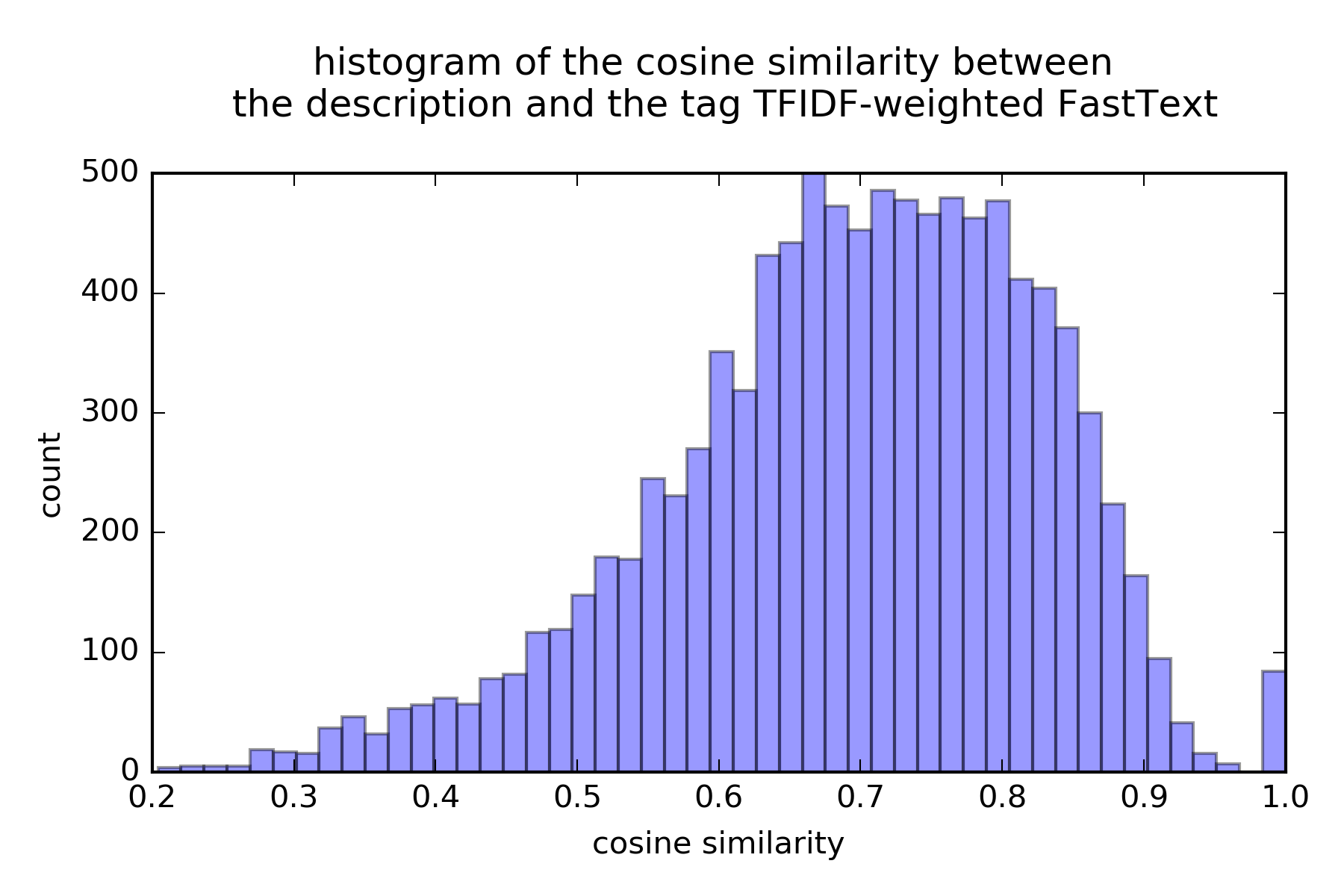
Figure 3.2. similarity between the X and Y TFIDF-weighted fastText.

5 Dimensionality Reduction

So at this point, we have the regressor which is a matrix of 10000,6837 dimesions. and the regressed as a matrix of 10000,701. We should be able to get a reasonable shot at the task. However, we still have one important step that we can improve on, which is dimensionality reduction. The advantages (shown in figure 4) that we observed are two folds, one is that the regression on the dimension reduced dataset is faster. Second is the dimensionality reduction acts as a de-noising method. Because distance measurement in very high dimensions suffers from “the curse of dimenionality”, the de-noising turns out to help the regression and improving the retrieval.

We pick a standard tool which is PCA as a way to reduce dimensionality of both the regressor and the regressed.

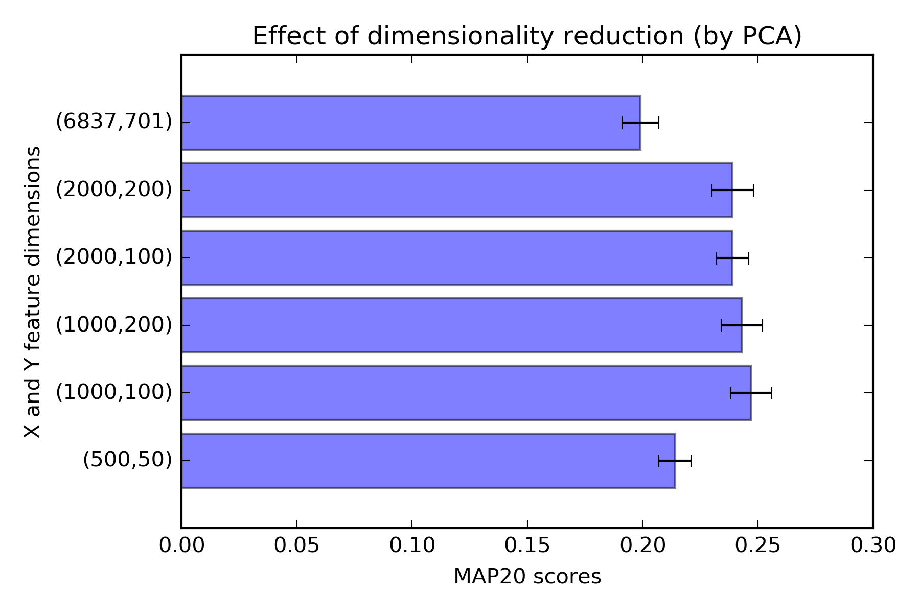
Figure 4. How PCA can help.

6. Ridge regression

Finally, we are ready to do the machine learning task. We perform 5 fold cross validation to estimate the MAP20 score. We use ridge (L2 regularization) regression because it is fast and easy to implement. The regularizatin regression is the minization of the least square residual term and the L2 regularization term aiming at penalizing the magnitude of the coefficients in the regression (thus reduce the over-fitting in case of regressions with too many regressors).

As it turns out, the limiting factor to our model is really the size of the training data. This is seen when we set different sizes of cross validation (see figure 5). So one obvious improvement for future work is to get more training data. The best cross validation score comes from the amulgamated model of PCA dimension-reduced text TFIDF, TFIDF-weighted fastText word2vec, and resnet-50 fastText. Interestingly, using TFIDF only is surprisingly well. This could be because the resnet-50 only classify object in the images into 1000 classes, while the human-generated text can be more fine-tuned or more specific.

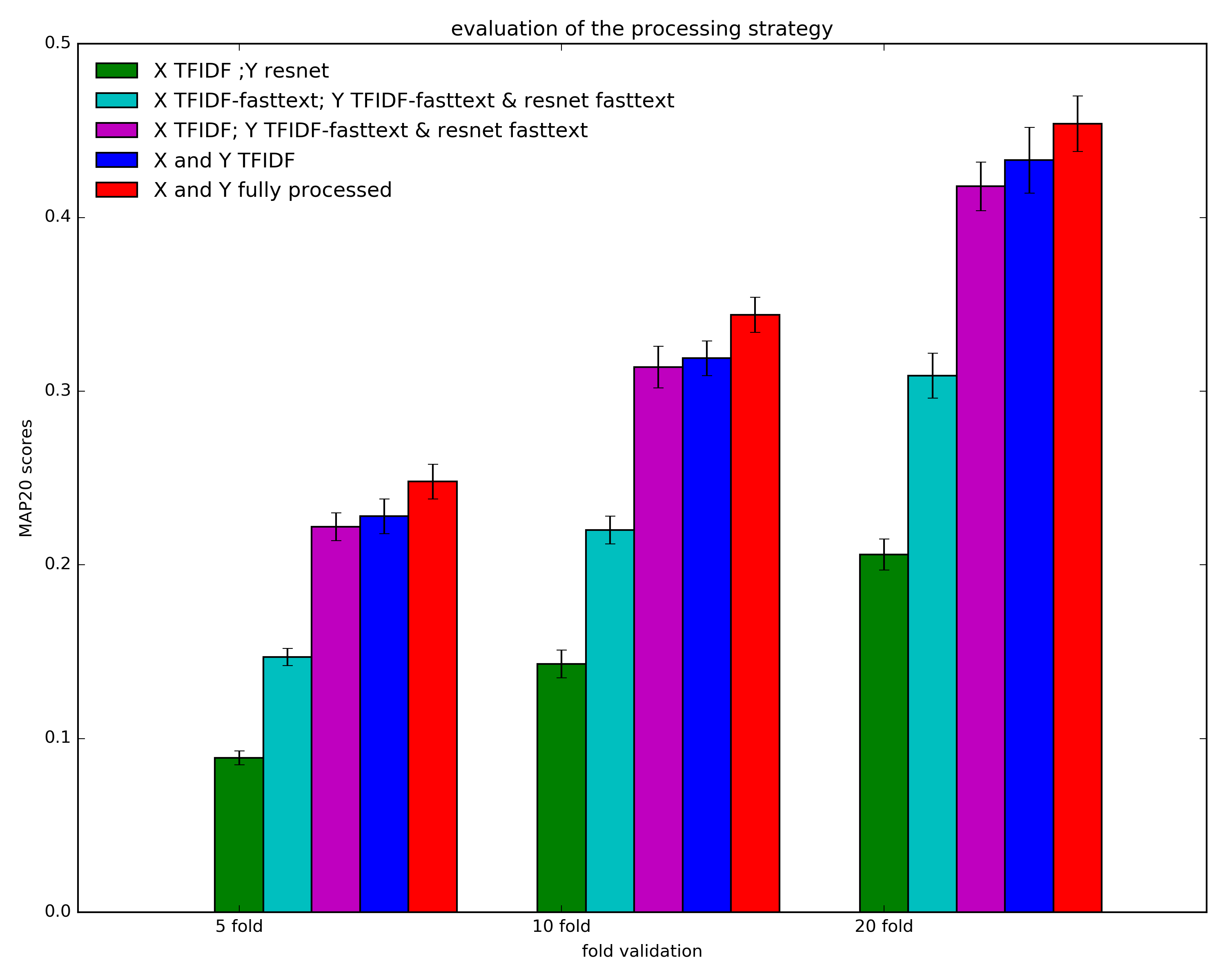
Figure 5. Evaluation of different processing strategy.

7. Result and Dicussion

To see how well our algorithm works, we look at how it ranks the correct images within the top 20 images it retrieves (see figure 6). As we can see, there are still a lot of images not correctly recalled within top 20 ranks.

Figure 6. ranks of correct images retrieved.

But now let’s see whether we can diagnose what kind of images are problematic, and what are pieces of cake for this algorithm.

The sets of figures below show the 5 sentence queries, and the top 20 image search results ordering from left to right, and top to bottom.

First of the figures below shows the 5 sentences and the image it gets right the first search.

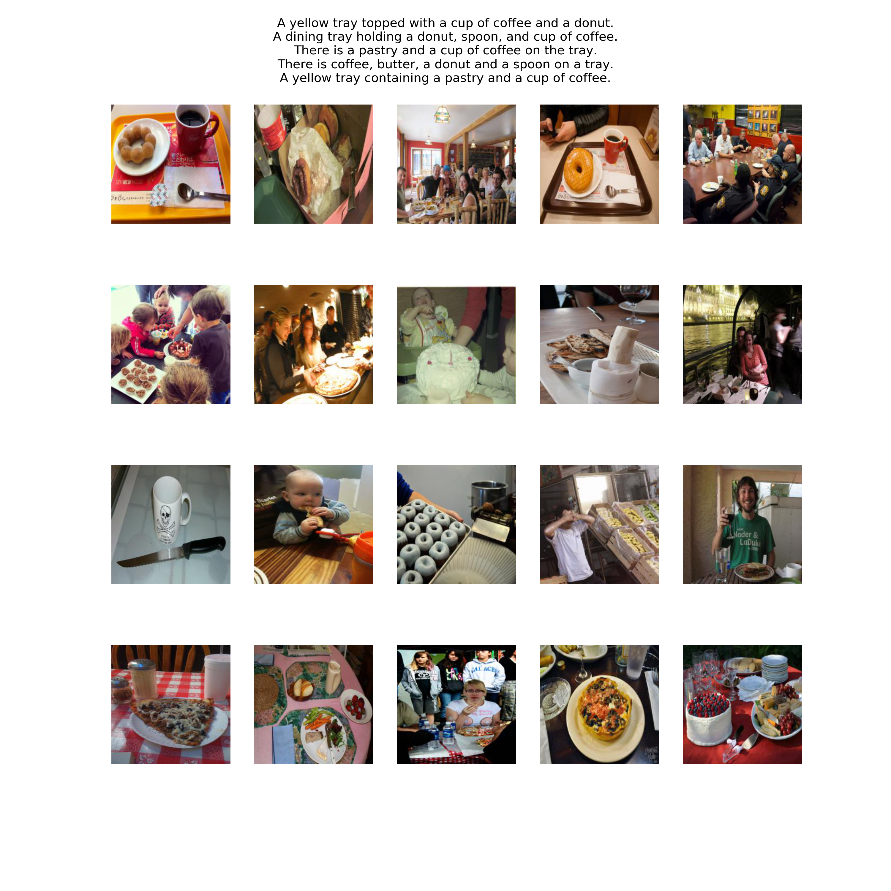
Figure 7. images retrieved at rank 0.

This is the example where the correct image is not within top 20 results.

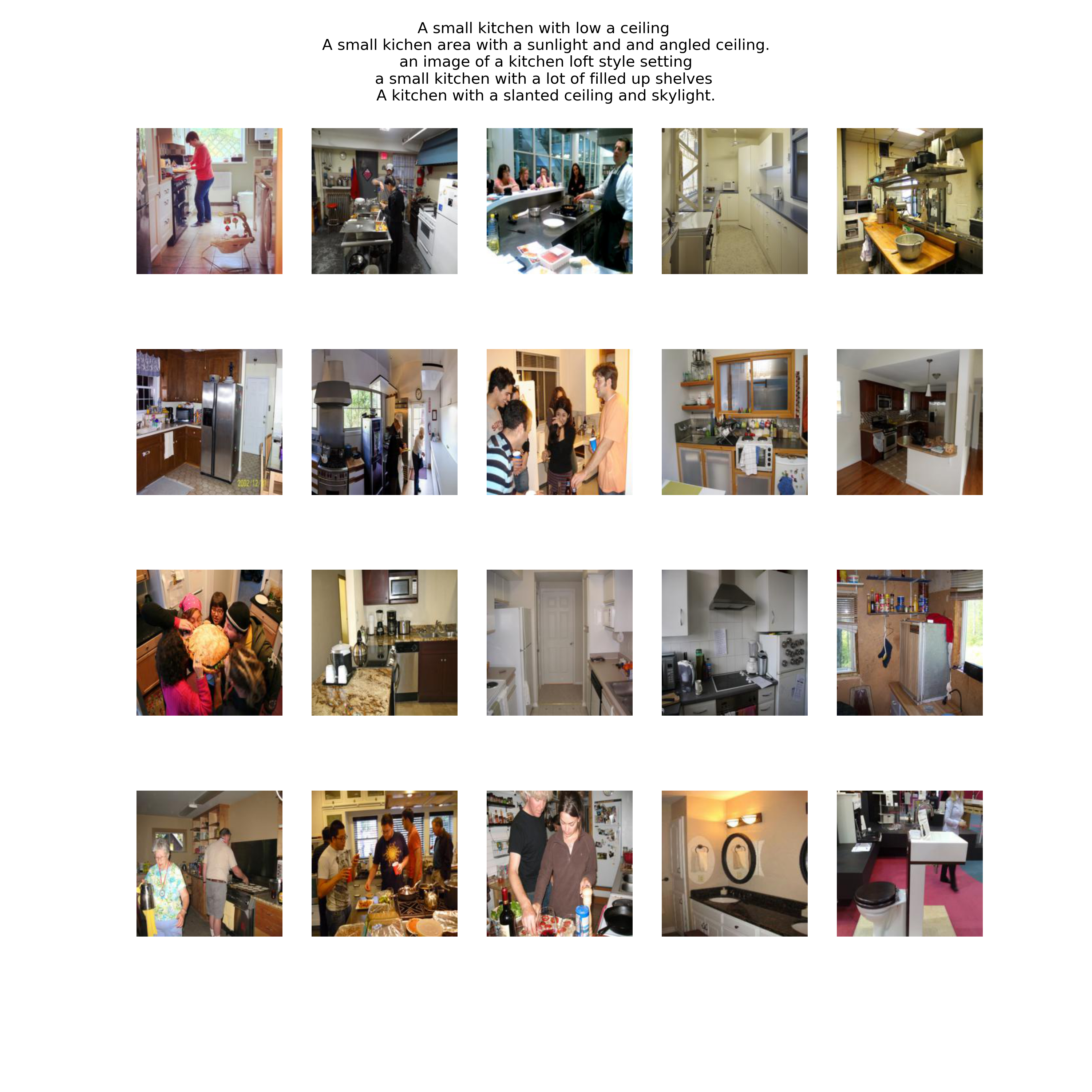
Figure 8.example 1 of mis-identification

And the correct image is shown here.

Figure 9. image of "A small kitchen with low ceiling".

In this case, we can say that all the images are too similar. One curious point is that the incorrect images contain a person/people in them, while the description does not mention people and the correct image does not contain people in it. The mis-identification happens because the TFIDF probably up-weigh the word “kitchen” but down-weigh “person”. And as a result, the algorithm picks out the images with kitchen, while ignoring the facts whether they have persons in the images. One future improvement is to develop further an algorithm that can discriminate images based on objects not found in the images and not mentioned in the text.

Another sort of problem that I see is that the description can be quite complicated. For example, this query is not retrieved.

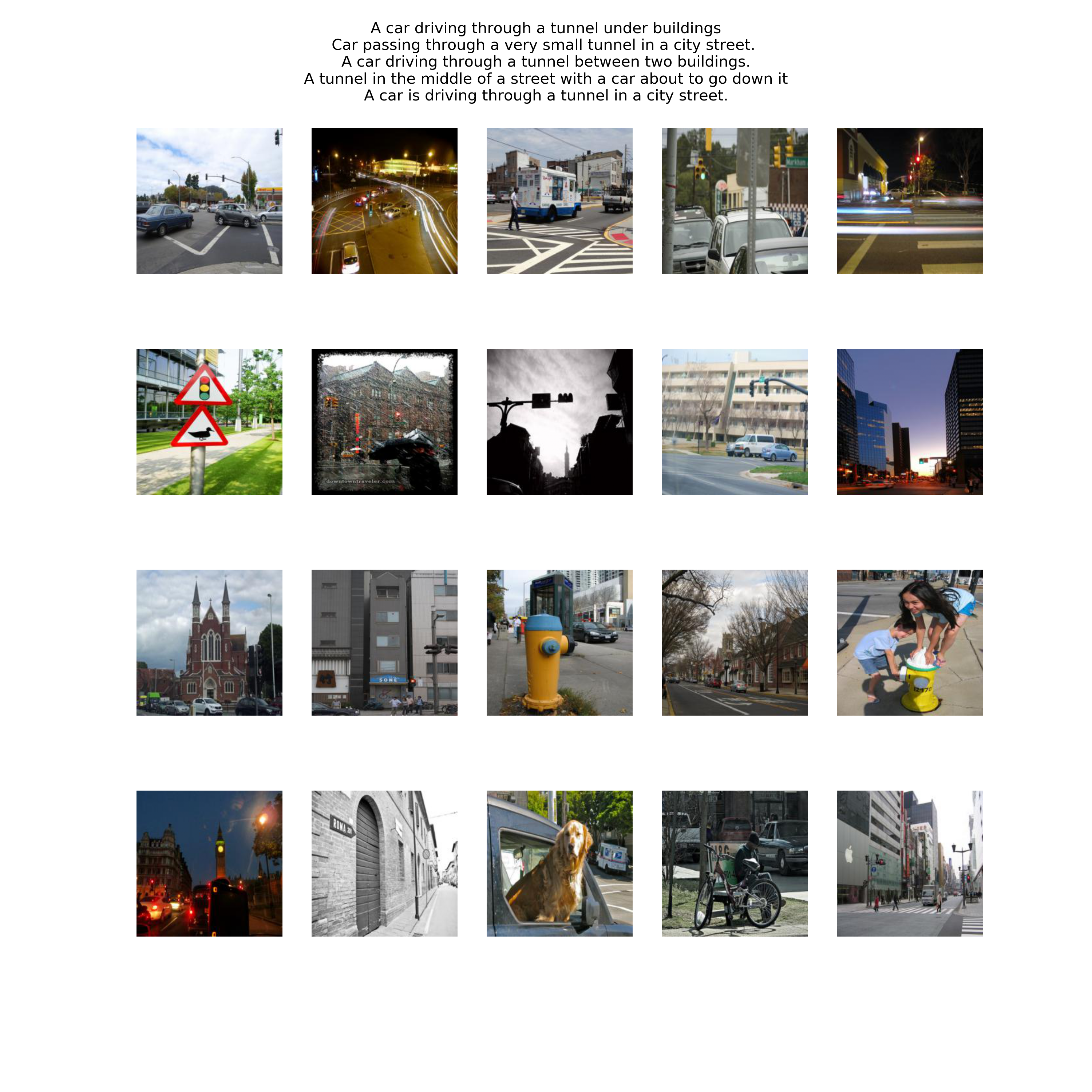
Figure 10. example 2 of mis-identification

And the correct image looks like this.

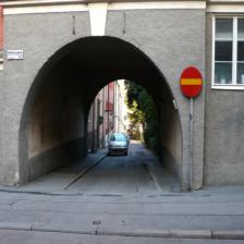
Figure 11. image of "A car driving through a tunnel under building".

What we see here is that there might still be information in the text at a level higher than word level (such as at the sentence level). Moreover, the ImageNet dataset only classify objects, and not actions (i.e. the results are all nouns, and not verbs). This can be what are missing in our algorithms and should be investigated in the future.

Appendix

1. ResNet

ResNet implements skip connetions that allows activation layers to feed forward into deeper layers. The advantage of this connection is to avoid the problem of vanishing/exploding gradients occured in very deep neural network. Roughly speaking, back-propagation in the neural network pass down the gradient (error signal) down the layer network by chain-rule. This has the effect of multiplying small gradients together, and decresing the values exponentially down the layer. If the layers are deep, the gradients can “vanish”, i.e. the signals are disappearing in the deep networks, making the training difficult.

The skip connection in ResNet solves this problem by sending the input signals along with the output signals to the next layers, so that even if the back-propagation causes gradients to drop to zero, the deep layers can still the identity input transfer back to the earlier layers, lessening the pain of vanishing gradients.Thus, ResNet allows training very deep neural network. I found this YouTube very helpful in understanding the issue.

2. FastText

Generally we want to transform words to vector representation, with the goal that word similarity is reflected as distance among vectors. To do the embedding we have to train a “word2vec” model, where large corpus of text is fed to a neural network model. The neural network task is to predicts words based on surrounding context. Roughly speaking, if two words are located around the similar context, and thus they are predictive of similar context, their “meaning” are related. Consequently, the vector representation of these two words are closer than the more unrelated words.

fastText is a related word2vec that is trained using skip-gram model, meaning each word is represented as sum of n-grams vector representations of characters. The advantage of this method above and beyond simple word2vec model is that it can handle out-of-vocabbulary words, such as rare words and technical terms.

3. TFIDF

Unlike, word2vec, the goal of TFIDF is to use statistics to find words that are more important in the document and are “representative” of the document. for example, if we want to classify whether documents are a food recipe or not, a term like “saucepan”, “saute”, or “stir try” would indicate that this is a document about food recipe. This is because the terms are found in food recipe and not much elsewhere.

IFIDF is a numerical method of weigh words in documents in a larger corpus based on this criteria. If words presents many times in small number of documents, these words give high discriminating power to those documents, and are up-weighted. Also, words that are presented in many documents, or simply rare and are not really give discriminating power to the documents are down-weighted.