Discoverying Advertising Adstock with Probabilistic Programming in Pyro

- Business Problem
- Problem formulation
- Solving the problem with Probabilistic Programming
- Probabilistic Programming
- Experiment
- Results
- Final Thought
- Citation
- Appendix
Business Problem
An important question in marketing data science is how media spend affects sales. I got the blog post idea from friends in data science who asks me my thoughts on the matter and gives me a paper to read.
This problem often comes up as “I spend money on day 1, when will I see the sales/subscriptions go up, and by how much”. The money spend now may take time to have an effect. For example, it might take some time for ads to circulate in the community. The effect of advertising may also carry over from one ads campaign to the next because people remember your products. This kind of effect is called a lag/carryover effect.
Another kind of effect has to do with the diminishing returns on ads. That is to say, spending too much on ads will simply saturate the market and any more money spent won’t drive the sales further. This is called saturation effect.
Ideally, marketers want to understand the two types of effects so that they can plan the spending at the right time at the right price. So in this blog post, I used probabilistic programming to find out the effects from simulated spend&sales/subscriptions data. I implemented the work in Pyro, a Pytorch-based tool in Python. The code can be found in the Appendix.
Problem formulation
Let’s formulate the problem. We start with the time series of spending&sales data. The sales driven by ads spending can be thought of as an effect of spending spead over a duration of time with some lag and carryover effect.
Mathematically, the lag period is represented as a delayed function and the memory retention is a decay function. This function, so-called adstock function, is best understood as a kernel or a density function that smooth the spending over time.
If we think that we are in the spending regime where the ads can saturate the market, we might need to quantify the diminishing returns on ads. Mathematically, this is as if the spending effect after the adstock function is passed through a non-linear function such as a logistic function, where the saturation effect is applied on top of the adstock effect. In this case, we will use Hill equation function as our saturation function. Hill equation has been used mostly in pharmacology for drug response effect. Nevertheless, the equation provides a general non-linear response curve applicable to our work.
To get a clearer picture, you can see the data generating code in the appendix subsection B and C as well as figure 1, 2, and 3.
Solving the problem with Probabilistic Programming
There are many possible ways to solve this problem. One way to deal with it is to recover the kernel from the spend data and the sales data. This could be done in a few lines of codes using machine learning tools such as neural network.
Another way to do this is to use Bayesian inference. The added benefit of doing this is that we get the full probability distribution of the adstock kernels. It provides the ranges and uncertainty estimates of the models.
Finally, the Bayesian inference could be done in a hierarchical manners where the kernel weight is generated from hyper-priors, namely the retention rate, delay rate, etc. This allows us to estimate the parameters such as delay, retention, etc. that govern the spending/sales dynamics.
I implemented all 3 approaches, using a single-layer neural network and Bayesian probabilitistic programming.
Probabilistic Programming
First before we go into the implementation details, let’s discuss probabilistic programming. Previously in this tutorial blog I tried to define probabilistic programming paradigm. Roughly speaking, probabilistic programming is a programming paradigm that aims at solving statistical models, mostly Bayesian statistics.
I found most active community of probabilistic programming in R or Stan. This is probably because academics use them. However, there are growing communities in Python as well, mostly around packages Pymc3 or Pyro.
There are a few pros and cons for using Pymc3 or Pyro.
| Pymc3 | Pyro | |
|---|---|---|
| community | pymc3 has been around longer and there are a lot more people using it. So you’re more likely to get help. | Pyro is newer. So the community is smaller. But it’s growing. |
| backend | Pymc3 uses theano backend. Theano has already been deprecated. | Pyro uses Pytorch backend. Pytorch is no. 1 package for deep learning. This alone is a good enough reason for me. |
| debugging | Theano documentation is not as good as Pytorch. I find it harder to debug, or understand what errors are telling me. | I’m more familiar with Pytorch. and the documentation is very well maintained. The error messages make sense. |
| visualization | Pymc3 has its own visualization. It can plot traces, computational graphs, distribution, etc. | Pyro currently does not have visualization built-in. I use matplotlib and seaborn. |
| prospect | tensorflow-backended Pymc4 will replace Pymc3 at some point soon. So Pymc3’s fate is up in the air. Tensorflow is a very good package for deep learning up there with Pytorch. So this is very exciting. | Pyro is too new. but definitely Pytorch is here to stay. |
The past log I did a Bayesian regression tutorial in Pymc3. So in this blog I’ll try Pyro. All the packages used in this work is specified in the appendix subsection A.
Experiment
The code for this part is in the appendix subsection B and C.
We will generate data at daily resolution for 365 days. The adstock function has maximum lag of 10 days, the retention rate of 0.85, and delay rate = 3 days. The saturation function has half saturation point = 1.6, slope = 10, and beta(multipler) = 1.5.
I found the saturation function is much harder to fit and need a lot of data. The data ideally should have enough varience to fit both the adstock (time delay+carryover) and the shape (saturation). So if the data is always saturated or never saturated, you’d see a trade-off between the adstock fitting and the shape fitting.
If you just wanted to fit the adstock kernel, you’d only need a few weeks of data. The decision whether to fit only the adstock, the saturation, or both depends on the quality of the data. Here I select parameters that allow me to effects and I use a lot of data.
This is what the spending and the sales (subscriptions) looks like for 90 days.
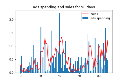
Figure 1. generated spending and sales data time series
One obvious thing to notice is that the peak spending and the peak sales are not aligned. The sales lags behind spending by a few days. The trough also lags behind. This is due to the adstock effect, both the delay and the retention effect. Another thing to note is that the spending effect is not linear. Around day 40, the peak ads spending does not result in proportionally higher sales. This is the saturation effect.
Below is what the adstock function looks like visually. This means spending at day 0 gets immediate 60% weight of effect. But the peak effect is delayed by 3 days; then it slowly decays down (each following day retain 85% of previous day’s effect).
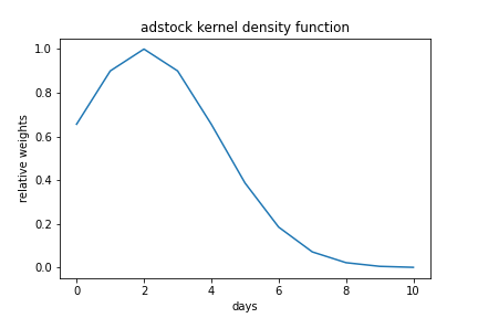
Figure 2. adstock showing the delay and the retention effect
Also here is the saturation function. I use Hill equation here as the saturation function. This allows me to specify the slope, the half-saturation point and the saturation value. But other sigmoid-shape functions should work also.
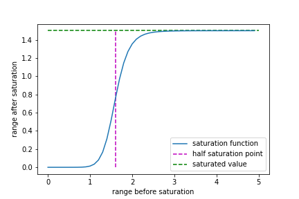
Figure 3. saturation function
Results
1. Discover the adstock effect using neural network.
Here we first look at a single layer neural network to for the adstock function. I tried both linear or fully connected (fc) and convolutional (conv) neural network. In both cases, I used pytorch implementation of neural network. The code for this part is shown in the Appendix subsection D.
I trained the model for 5000 iterations. The results shown below are the weights of the neural network used to fit it. The weights should reflect the adstock kernel, which they indeed are.
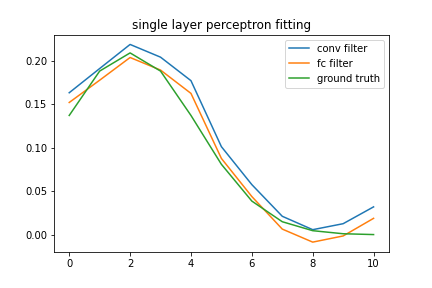
Figure 4. adstock kernel compared to the fitted models
2. Using Bayesian inference to estimate the adstock effect
Let’s say we need to quantify uncertainty in the adstock kernels. We can implement Bayesian inference to get the full distribution of the adstock function.
The code for this part is included in the appendix subsection E.
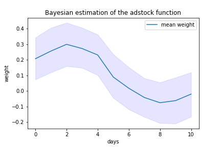
Figure 5. Bayesian inference of the adstock function. The shaded area represents 90% credible interval.
To get a better estimate, we’d probably need more data, or provides a better regularization of the adstock, which leads us to the next section.
3. Using Bayesian inference to estimate the the parameters of adstock + saturation
In the last section, I used Bayesian inference to estimate the weights of the adstock kernel directly. The weight of each day is sampled from a normal distribution independently from the weight of other days.
But we can do better than that. I hypothesize that the adstock weights are generated from a specific adstock function. So they are in fact not independent from one day to the next. It would be better to model the adstock function itself. The number of parameter we’d estimate will be smaller. In addition, it would give us more constraint on the shape of the kernel.
The code is included in the appendix subsection F.
In this section, I specified the parameters of both the adstock and the saturation functions, then let the Bayesian inference estimates the values of those parameters.
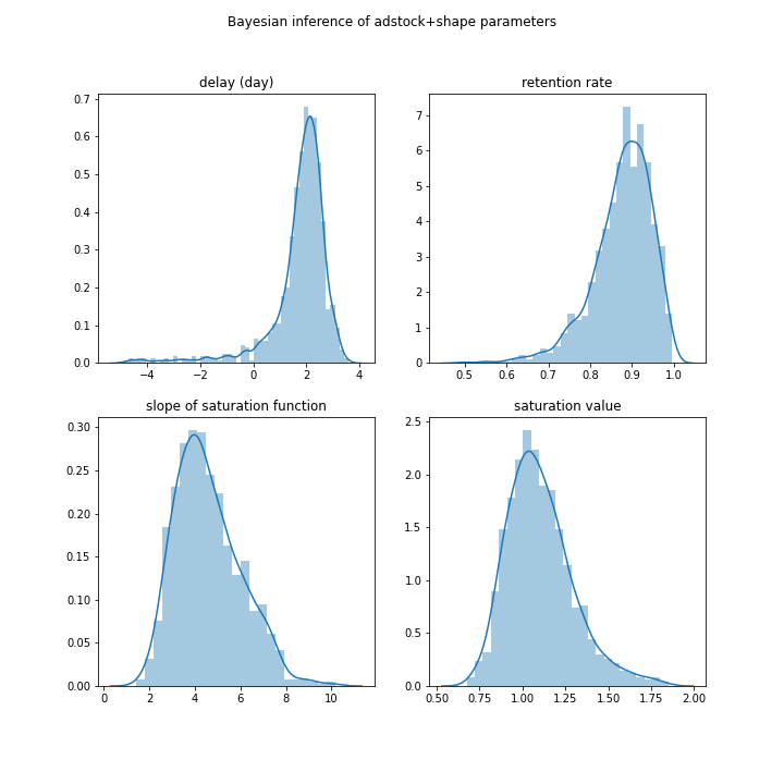
Figure 6. Bayesian inference of the adstock and saturation function. The histogram shows the distribution of the parameters.
Here we can say that the inference captures the parameters for the adstock correctly. But the saturation function still has the wrong shape. This is not too disappointing as I said earlier that the saturation function is much harder to recover.
Now let’s turn our attention to the adstock function estimate. Comparing the figure 7 to figure 5, we see that the credible interval of the figure 7 is narrower. This fits our prediction in the beginning.
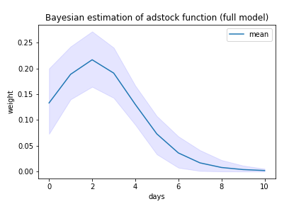
Figure 7. Bayesian inference of the adstock function parameters.
Finally, we look at the saturation function.
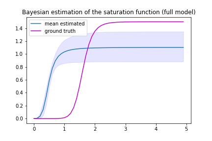
Figure 8. Bayesian inference of the saturation function.
Here I show the diminshing return, and it has the correct shape. However, the prediction gets the saturation value off. The ground truth value is higher.
Final Thought
Here I showe how we can use probabilistic programming package Pyro to write a Bayesian model to quantify the ads spending.
In all cases, we specify maximum lag time to be the actual maximum lag time that the data is generated from. Now in reality, this is not known. So we’ll have to try a few lag time and see which lag time best fits the models. The idea is that if we specify too short lag time, we will not be able to recover all the adstock effect. If we choose lag time too long, we won’t gain any more information, but may overfit the model. By comparing the performance of different models, we should be able to identify the appropriate lag time. All the codes are in place, so I leave this as a homework for readers to work this out.
In the end, I feel that choosing a good starting prior well will really help you get a good estimate. This is because the complex model is numerically unstable, and can be very sensitive to priors. This is where domain expertise can comes into the picture. Experts would probably have a sense about what plausible ranges of values are for the adstock and saturation.
I realize at the end of writing that this work is probably going to be a part of a larger work on media mixed model. I’ll be working on a simplistic marketing attribution model next. So stay tune.
Citation
-
paper This is the paper by Google that outline Bayesian inference for adstock function. The work is done in Stan though. So I didn’t follow the method line-by-line in Pyro.
-
Pyro This is the main Pyro website that keep the documentation and a few example codes.
Appendix
A. packages
packages you'd need
import matplotlib.pyplot as plt
import seaborn as sns
import numpy as np
import pandas as pd

import torch
import torch.nn as nn

!pip3 install pyro-ppl==1.3.1
import os
import pyro
import pyro.distributions as dist
pyro.set_rng_seed(1)
pyro.enable_validation(True)
from pyro.infer import MCMC, NUTS
from pyro.nn import PyroModule, PyroSample
B. helper function
Here below are all the helper functions that we’ll need to generate the dataset. Note here that we will be working with a padded matrix of size M,N where M is size of dataset and N is the maximum lag we are interested in.
helper functions
def get_padded_spend(spend, max_lag):
    """
    convert vector of spend/impressions to matrix where
    each column is one element with
    [spend[t], spend[t-1], …, spend[t-max_lag]]
    shape = (day x max_lag)
    """
    X_media = []
    N = len(spend)
    for time_point in range(N):
        unpadded = spend[max([0, time_point-max_lag]):(time_point + 1)]
        pad = [0]*max([0, max_lag + 1 - len(unpadded)])
        X_media.append(unpadded[::-1] + pad[::-1])
    return np.array(X_media)

def get_delayed_adstock_weights(retain_rate, delay, max_lag):
  """
  spread the effect of advertizing spend (i.e. weights of adstock) over time
  the effect is carried over from time t to t+1 at retain_rate
  the peak can be delayed (delay term)
  and the effect lasts max_lag
  """
  lag = np.arange(0, max_lag + 1)
  return retain_rate**((lag-delay)**2)

def adstock_transform(X_media, adstock_weights):
  """
  This function applies the carryover effect to the spending data.
  1. exposure today has effect in the future
  2. effect decays over time

  apply the adstock weights to the spend period data
  """
  return (X_media.dot(adstock_weights))/sum(adstock_weights)

def get_hill_function(x, ec, slope):
  """
  This function generates shape effect to the effect
  1. effect of exposure is subjected to the law of diminishing returns
  2. changing the level of ad exposure brings about relative change in sales volumes

  to get the shape effect, put the media spend data throuh curvature transformation
  i.e. gives the saturation effect
  ec = ec50 of half saturation point
  slope = shape parameter
  """
  if any(x < 0):
      raise ValueError("x must be > 0.")
  return 1/(1+ (x/ec)**-slope)
C. Generating data example
generate data
def generate_data(period,max_lag,retention,delay,ec50=0.5,slope=1.0,beta=0.5,add_saturation=False,sigma=0.1):
  list_spend = []
  for i in range(period):
    list_spend.append(np.random.exponential(0.5)) # the spending is sampled from exponential distribution
  matrix_spend = get_padded_spend(list_spend,max_lag)
  kernel_adstock = get_delayed_adstock_weights(retention,delay,max_lag)
  response = adstock_transform(matrix_spend,kernel_adstock)
  response = response + np.random.normal(1,sigma,size=len(response))
  if add_saturation:
    saturated_response = beta*get_hill_function(response,ec50,slope)

  x_data = torch.Tensor(matrix_spend)
  y_data = torch.Tensor(response)
  z_data = torch.Tensor(saturated_response)

  return x_data, y_data,z_data,kernel_adstock, list_spend

carryover_X, carryover_y,carryover_sat, kernel_carryover,list_spend = generate_data(365,10,0.9,2,
                                                                  ec50=1.6,slope=10,beta=1.5,add_saturation=True)
D. Use Pytorch to discover an adstock kernel
Here we will write 2 single layer perceptrons (neural networks) to fit the adstock function. First model is a linear model. Second model is a convolutional model. For each one, we’d need to specify the loss function and the optimizer. We’ll use mean square loss and Adam optimizer. We’ll train the model for 5000 iterations. It should be done almost instantly.
model = nn.Linear(11,1)
model = model.to(device)
learning_rate = 1e-3
criterion = torch.nn.MSELoss()
optimizer_fc = torch.optim.Adam(model.parameters(), lr=learning_rate)

conv_model = nn.Conv1d(1, 1, 11, stride=1)
learning_rate = 1e-3
criterion = torch.nn.MSELoss()
optimizer_conv = torch.optim.Adam(conv_model.parameters(), lr=learning_rate)

def execute_function(model,optimizer,epochs, data_X, data_y,conv=False):
  epoch_loss = []
  count = 0
  if conv:
    data_X = data_X.unsqueeze(0).unsqueeze(0)
  for epoch in range(epochs):
    temp_loss = []
    model.train()
    optimizer.zero_grad()
    result = model(data_X)
    #print(result.shape)
    if conv:
      result = result.squeeze(0).squeeze(0)
    else:
      result = result.squeeze(1)
    loss = criterion(result,data_y)
    loss.backward()
    optimizer.step()
    temp_loss.append(loss.item())
    count += 1
    #print(count)
    epoch_loss.append(np.mean(temp_loss))
  return epoch_loss

torch_spend = torch.Tensor(list_spend)

loss1 = execute_function(conv_model,optimizer_conv,5000,torch_spend,carryover_y[10:],conv=True)

loss2 = execute_function(model,optimizer_fc,5000,carryover_X,carryover_y)

 # to plot this we can get the weights of the models and plot the weights
 # note the conv. filter is the flipped kernel due to the notation convention of convolution.
 # we will just flip back
 # below here is the code plotting

conv_filter = conv_model.weight.squeeze(0).squeeze(0).detach().numpy()[::-1]
np_kernel = model.weight.detach().numpy()
np_kernel = np_kernel.reshape(11)
plt.plot(conv_filter,label = 'conv filter')
plt.plot(np_kernel,label='fc filter')
plt.plot(kernel_carryover/np.sum(kernel_carryover),label = 'ground truth')
plt.legend(loc='best')
plt.title('single layer perception fitting')
E. Use Pyro to get an adstock kernel
Here in this section. we’ll write a Pyro model to sample the adstock kernel weights from distributions. Then we’ll fit the model using Hamiltonian Monte Carlo algorithm.
 # first we will specify the model as function
 # this is different from Pymc3 which uses with context manager

def bayesian_model_indexing(x_data,y_data,max_lag=11):
  # the weights (shape = 11) are sampled independently from 11 normal distribution.
  weight = pyro.sample('weight',dist.Normal(torch.zeros(max_lag),5.0*torch.ones(max_lag)))
  with pyro.plate('data',len(x_data)):
    mean = torch.sum(weight*x_data,dim=1)  # apply adstock kernel to the spend data (dot product)
    pyro.sample('y',dist.Normal(mean,1),obs=y_data) # the result is the sales. subjected to observation


 # Then we will call create NUTS and MCMC objects which specify how we will run MCMC
kernel_bayes= NUTS(bayesian_model_indexing)
mcmc_bayes = MCMC(kernel_bayes, num_samples=1000, warmup_steps=200)
mcmc_bayes.run(carryover_X, carryover_sat) # don't forget to include your data in the run

 # we get the traces of MCMC and store as a dictionary
 # we then can use these traces to find means and credible intervals
 hmc_samples = {k: v.detach().cpu().numpy() for k, v in mcmc_bayes.get_samples().items()}

 # get the means value, and 90% credible interval
mean_weight = np.mean(hmc_samples['weight'],axis=0)
weight_0p1 = np.quantile(hmc_samples['weight'],q=0.1,axis=0)
weight_0p9 = np.quantile(hmc_samples['weight'],q=0.9,axis=0)

 # finally we can plot this in Matplotlib
fig, ax = plt.subplots()
ax.plot(mean_weight,label='mean weight')
ax.fill_between([i for i in range(11)],weight_0p1,weight_0p9, color='b', alpha=.1)
ax.legend(loc='best')
plt.title('Bayesian estimation of the adstock function')
plt.xlabel('days')
plt.ylabel('weight')
F. Discover the Adstock function parameters using Pyro
Finally, we can write a hierarchical model that samples the adstock parameters that in turns specify the adstock kernel. We will then again fit the model using Hamiltonian Monte Carlo.
def bayesian_model_adstock(x_data,y_data,max_lag=15,fit_Hill=False):
  lag = torch.tensor(np.arange(0, max_lag + 1))
  # here instead of sampling weights, we will sample the adstock parameters
  # the parameters are sampled independently from normal distribution
  retain_rate = pyro.sample('retain_rate',dist.Uniform(0,1))
  delay = pyro.sample('delay',dist.Normal(1,5))

  # the adstock parameters are used to generate the adstock kernels
  weight = retain_rate**((lag-delay)**2)
  weight = weight/torch.sum(weight)

  # sample the saturation function parameters
  ec50 = pyro.sample('ec50',dist.Normal(0.5,1))
  slope = pyro.sample('Hill slope',dist.Normal(5,2.5))
  beta = pyro.sample('beta',dist.Normal(0,0.5))

  with pyro.plate('data',len(x_data)):
  	# apply adstock kernel to spend data
    mean = torch.sum(weight*x_data,dim=1)
    # conditional, do you want to fit saturation function ?
    if fit_Hill:
      response = 1/(1+ (mean/ec50)**-slope)
      response = beta*response
    else:
      response = mean
    # the result is the sales which is subjected to the observation.
    pyro.sample('y',dist.Normal(response,1),obs=y_data)

kernel_bayes= NUTS(bayesian_model_adstock)
mcmc_bayes = MCMC(kernel_bayes, num_samples=1000, warmup_steps=200)
mcmc_bayes.run(carryover_X,carryover_sat,max_lag=10,fit_Hill=True)

hmc_samples = {k: v.detach().cpu().numpy() for k, v in mcmc_bayes.get_samples().items()}